Speech Enhancement using Deep Learning (3/4) - The Denoising Autoencoder
Goal and rationale
We have now arrived at part three of this series on speech enhancement using deep learning. While the previous two parts, admittedly, had nothing to do with deep learning (DL), we will now finally live up to the title of this series. In this part, we will rebuild a classic DL architecture for speech enhancement: the denoising autoencoder (DAE). And while we are at it, we will also revisit the concept of latent representations, that are the conceptual backbone of autoencoders.
Of course, we will thoroughly cover the entire MLOps pipeline for this project, from data collection and preprocessing, to model training and evaluation. But before we get into the nitty-gritty details of the implementation, let’s first take a step back and understand what a denoising autoencoder is, and why it is useful for speech enhancement.
We will cover the following topics in this part:
- A recap of autoencoders and latent representations
- The data we will use for training our model
- The audio preprocessing and feature extraction pipeline
- Neural network architecture
- Coding and training the model
- Evaluation and results
For the impatient: I will rebuild the DAE architecture (d) from Nossier et al. (2020), which is a simple feedforward autoencoder that takes log magnitude spectrograms as input, and has a remarkably good performance on speech enhancement tasks (but uses a whopping 2.0 million parameters).
Recap: Autoencoders and latent representations
An autoencoder is a special neural network architecture that is trained to reconstruct its input. Now, why would anyone want to do that? Could you not just use the input as the output, and you would have a perfect reconstruction? Well, yes, but that would not be very interesting. The magic of autoencoders lies in the fact that we force the network to learn a compressed representation of the input, called the latent representation, by introducing a bottleneck in the architecture (see Fig. 1). This bottleneck forces the network to compress the input into a lower-dimensional space, from which it can then reconstruct the original input. The hope is that this compressed representation captures the most salient input features.
The autoencoder was discovered in 1986 by Rumelhart et al., and was a major breakthrough in the field of representation learning. It showed that neural networks could learn useful representations of data, and paved the way for many neural network architectures we use today.
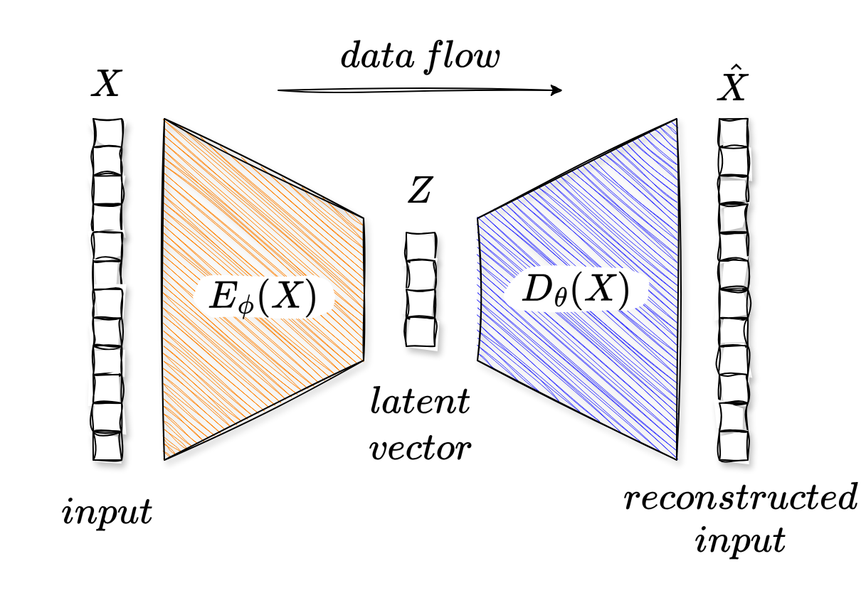
Fig 1. - A simple autoencoder architecture. The input is compressed into a latent representation, and then reconstructed back to the original input. Image by author (download draw.io template).
Let’s disassemble the architecture. An autoencoder consists of two main components: the encoder and the decoder. The encoder is a parameterized function, typically a neural network, that maps the input data to a latent representation. Following the structure from the figure above, we can denote the encoder as a function with parameters , that takes an input and maps it to a latent representation :
From the latent representation , the decoder, which is another parameterized function (also typically a neural network), maps back to a reconstruction of the original input, which we can denote as :
During training, the parameters of the encoder and decoder are optimized to minimize the reconstruction error between the original input and the reconstructed output . This is typically done using a loss function such as mean squared error (MSE):
So far, so good. Let us now see how we can put this architecture to work for speech enhancement.
The Denoising Autoencoder
The Denoising Autoencoder (DAE) was first introduced by Vincent et al. in 2008, and is a variant of the standard autoencoder that is trained to reconstruct clean inputs from corrupted versions of the data. Let’s build a mental model quickly.
Instead of feeding clean data into the autoencoder, we first corrupt it with some noise to get a noisy version . The DAE is then trained to reconstruct the original clean data from the noisy input. The architecture of a DAE is shown in Fig. 2.
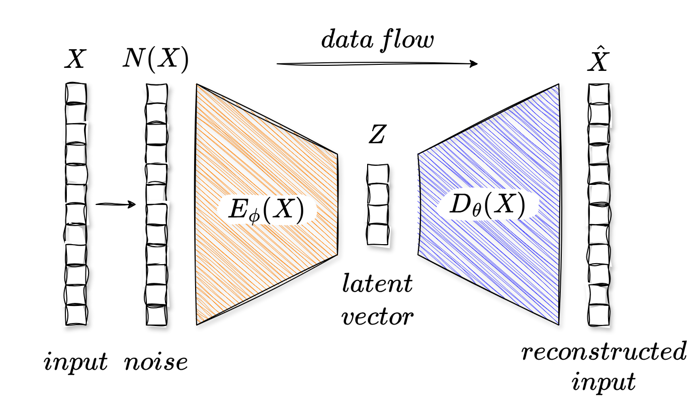
For our speech enhancement task, what we hope to achieve with this architecture is, that the encoder maps a noisy speech signal to a latent representation that captures the underlying structure of human speech from which the decoder can then reconstruct a clean version of the input speech signal. Let’s see how far this will get us in practice.
The dataset
Now, since we are in a deep learning context, we obviously need a dataset to train our model on. In fact, if we recall the DAE architecture from above, we actually need two datasets: one that contains clean speech signals, and another that contains noise signals for us to mix with the clean speech to create our noisy inputs. Due to the fact that we will train our model on the reconstruction loss between the clean input signals and the reconstructed outputs, we have to employ this pre-mix processing step, as otherwise we would not have access to the clean signals during training.
There is a multitude of speech and noise datasets available, specifically designed for speech enhancement (see Table 3 of Jannu et al. (2025)). For this project, I chose the following (freely available) datasets:
-
For clean speech, I will use the LibriSpeech dataset from Panayotov et al. (2015). This dataset contains approximately 1000 hours of clean speech from audiobooks sampled at 16 kHz, and is widely used in the speech processing community. What I like about this dataset is that it contains subsets of varying sizes, so one can easily scale up the amount of data used for training. And second, it has a high variety of over 1000 speakers, which is important for training a robust model. To keep things simple, I will only use the “train-clean-100” subset, which contains 100 hours of clean speech.
-
For noise, I will use the DEMAND dataset from Thiemann et al. (2013). This dataset contains recordings of various types of noise sampled at 16 kHz, such as street noise, cafe noise, and office noise, which are commonly encountered in real-world scenarios. As a fun fact, for each environment, the noise was actually recorded with a 16-channel microphone array, so you can also use this dataset for Acoustic Source Localization (ASL) tasks. For our purposes, however, we will only use the first channel of the recordings.
To give you an idea what we are dealing with, here is one example of a clean speech signal from the LibriSpeech dataset, and one example of a noise signal from the DEMAND dataset:
Aud. 1. - An example of a clean speech signal from the LibriSpeech dataset.
Aud. 2. - An example of a (METRO) noise signal from the DEMAND dataset cut to 10s of length. To showcase the noise, its loudness was increased via an integrated EBU R128 normalization (-24 LUFS).
Since both the clean speech and the noise recordings are single-channel audio files, our model will necessarily be a single-channel model. We therefore perform monaural speech enhancement.
Audio preprocessing and feature extraction
With our datasets in place, we can now just mix the clean speech and noise signals together, and feed the resulting noisy signals into our DAE. Right? Not too far off actually. I did some literature research on the topic and came across two different methodological approaches:
-
Working with spectral features, such as the magnitude spectrogram, log-mel spectrogram (we will cover this later), Gabor filter bands etc., which are derived from the STFT of the audio signal. This is, still to date, a common approach in the literature, and has been shown to work well for speech enhancement tasks.
-
Working with the raw audio signal directly, which is also known as end-to-end speech enhancement. This approach has gained popularity in recent years, especially with the advent of powerful neural network architectures such as convolutional neural networks (CNNs) and recurrent neural networks (RNNs), that can effectively model the temporal structure of audio signals (See for example SEGAN by Pascual et al. (2017) or the Wave-U-Net by Stoller et al. (2018)).
We now arrived at an architectural crossroads, but for the sake of applying at least parts of our newly acquired knowledge on spectral representations and the DFT, we will go with the first approach, and work with the log magnitude spectrograms of the audio signals. Specifically, I chose to rebuild the DAE architecture (d) from Nossier et al. (2020), as it is both straightforward to implement, and has been shown to perform well on speech enhancement tasks compared to other DAE architectures.
The log-magnitude spectrogram
Mathematically the log-magnitude spectrogram can be derived from a time-domain audio signal with only operations we have already covered in the previous parts:
where denotes the DFT of the signal . While the idea of the log-magnitude spectrogram is straightforward, there remain implementation details that we need to figure out. Currently, I see three main questions:
- Why do we take the logarithm of the magnitude spectrogram? What is the rationale behind this operation, and how does it affect the training of our DAE?
- What should our look like? What size is it, what about spectral leakage, and how do we handle the temporal dimension of the spectrogram?
- If we only use the magnitude spectrogram, we are discarding the phase information of the audio signal. How does this affect the quality of our reconstructed audio signal, and is there a way to mitigate this issue?
Logarithms?
The answer to the first question lies in the way we humans perceive sound. The human auditory system perceives sound logarithmically, meaning sensitivity to frequency shifts is significantly higher at lower ranges. For example, a shift from 40 Hz to 80 Hz is perceived as a much larger interval than a shift from 4000 Hz to 4040 Hz, despite the identical 40 Hz magnitude. Treating all frequency bins equally in a spectrogram would cause a neural network to disproportionately prioritize high-frequency accuracy, where errors are less perceptible, while neglecting the low-frequency details critical to speech. By applying a logarithmic transformation to the magnitude spectrogram, we compress its dynamic range and align the model’s objective with human perception, ultimately enhancing the performance of the DAE.
Input shape
The second question involves an implementation detail that serves as the bridge between theory and practice. While it might seem intuitive to simply take a raw audio signal , compute its Discrete Fourier Transform (DFT), and use the log-magnitude as input, this approach is flawed for two primary reasons:
-
Temporal Practicality: The DFT is defined for finite-length signals. Using a single DFT would require knowing the exact start and end of a signal beforehand. This is impossible for real-world data streams: imagine a phone call where you couldn’t hear the speaker until they hung up.
-
Architectural Constraints: Neural networks generally require fixed-size inputs. Since audio clips vary in duration, a global DFT would yield varying input dimensions, which modern architectures cannot natively handle.
The solution is the Short-Time Fourier Transform (STFT). By dividing the signal into short, equal-length “frames” (typically in the millisecond range) and computing the DFT for each, we transform the temporal dimension into a series of manageable snapshots.
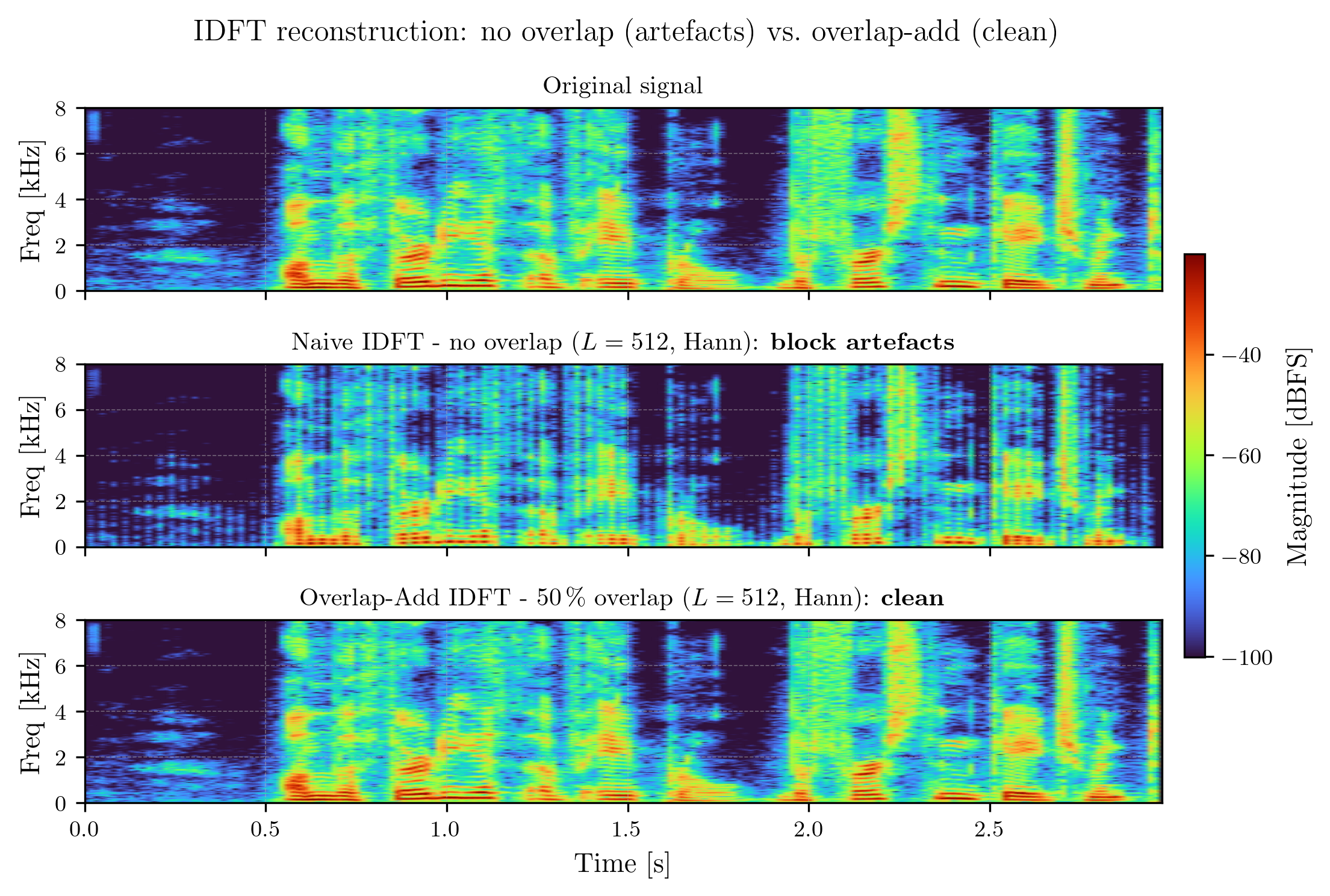
However, this introduces the issue of spectral leakage. As we discussed in Part 2, “glueing” raw segments together creates discontinuities that manifest as noise in the frequency domain. To mitigate this, we apply a window function (like Hann or Hamming) to each segment, tapering the signal toward zero at the edges.
While windowing solves the leakage problem, it introduces a new one: by tapering the edges, we effectively discard information at the start and end of every frame. To ensure no data is lost and to allow for perfect reconstruction, we employ Overlap-Add (OLA). By overlapping these windows - a distance defined by the hop size - we ensure that the “faded” information in one window is captured at the peak of the next. You can see the impact of this reconstruction technique on a random sample from the LibriSpeech dataset in Figure 3 below.
You can listen to the reconstructed audio signals too:
Aud. 3. - The reconstructed audio signal without overlap-add, which contains artifacts due to spectral leakage.
Aud. 4. - The reconstructed audio signal with overlap-add, without artifacts.
We are now only missing values for all of the parameters of the STFT. I will provide them right after answering question three.
Phase information
The third question addressing the phase information presents a more complex challenge. By focusing solely on the magnitude spectrogram, we discard phase data essential for high-fidelity signal reconstruction - a challenge widely recognized as the “phase problem.” Because phase is notoriously difficult to model, most enhancement frameworks focus on the magnitude while leaving the original phase unaltered. However, this oversight often introduces audible artifacts, such as musical noise. A common mitigation strategy is to combine the enhanced magnitude with the phase of the noisy input signal. While effective in many scenarios, this heuristic remains imperfect and may still produce artifacts, particularly in low- (Signal-to-Noise Ratio) environments. While advanced methods like complex-valued neural networks offer more robust phase modeling, they remain beyond the scope of our project. For our DAE, we will therefore adopt the common practice of using the noisy phase during reconstruction, while acknowledging the limitations this imposes on the quality of our enhanced audio.
The features
With all of the above in mind, we can now define our input features for the DAE. To ease us with computation, all audio signals will be resampled to a common sampling rate of 8 kHz. We will compute the log-magnitude spectrograms of our audio signals using the following parameters for the STFT according to Nossier et al. (2020):
| Parameter | Value | Rationale |
|---|---|---|
| Window size | 256 samples (32 ms) | A larger window size provides better frequency resolution, which is important for capturing the harmonic structure of speech. However, it also reduces temporal resolution, which can make it harder to capture transient events. A window size of 256 samples strikes a good balance between frequency and temporal resolution for speech signals. |
| Hop size | 128 samples (16 ms) | A smaller hop size provides better temporal resolution, which is important for capturing the dynamics of speech. However, it also increases the computational cost, as we have to compute more STFT frames. A hop size of 128 samples is a common choice for speech processing tasks, as it provides good temporal resolution while keeping the computational cost manageable. |
| Window function | Hanning window | The Hanning window is a commonly used window function that helps to reduce spectral leakage by tapering the edges of each window towards zero. It is a good choice for speech signals, as it provides a good balance between mainlobe width and sidelobe level, which helps to preserve the harmonic structure of speech while minimizing leakage. |
How to add the noise?
To create our noisy input signals for training the DAE, we will mix the clean speech signals from the LibriSpeech dataset with the noise recordings from the DEMAND dataset at various Signal-to-Noise Ratios (SNRs). The SNR is defined as the ratio of the power of the clean signal to the power of the noise, and is typically expressed in decibels (dB):
where the power of a signal is defined as the mean squared value of the signal:
For a given SNR value, we can compute the required noise power to achieve that SNR via
and derive the scaling factor for the noise signal as
The square root is necessary because we are working with power, which is proportional to the square of the signal amplitude (), and since we eventually want to scale the amplitude of the noise signal, we need to take the square root. By scaling the noise signal by , we can ensure that the resulting noisy signal has the desired SNR when mixed with the clean signal.
Putting everything together, we can create our noisy input signals for training the DAE as follows:
Implementation detail: To avoid clipping the combined signal, we peak-normalize:
Neural network architecture
I will roughly follow the architecture of the DAE (d) from Nossier et al. (2020), which is a feedforward autoencoder. The encoder consists of three fully connected layers with ReLU activations, and Layer Normalization. The hidden layer sizes are [2048, 500], the bottleneck layer has a size of 180, and the decoder is a mirror of the encoder with hidden layer sizes [500, 2048]. The output layer has the same size as the input layer, which corresponds to the number of frequency bins in the log-magnitude spectrogram.
There are two things that differ from the original architecture: first, I will not use dropout, as I found that it does not improve the performance of the model in my experiments. Second, I will use Layer Normalization instead of Batch Normalization.
I do not really have empirical justification for using Layer Normalization instead of Batch Normalization, but from a conceptual standpoint it seems much worse in my opinion to normalize across randomly selected small batches, or to estimate centering and scaling factors using exponential moving averages, than to just normalize across layers.
Coding and training the model
Okay, so finally we have all the pieces in place to code and train our DAE. I will use PyTorch for this implementation, not only for the networks but also for the datasets.
All the code presented here, is done without too much doc strings inside the code itself, to improve readability. However, I will provide you with a fully documented version of the code in the GitHub repository for this project, which you can find here. The accompanying documentation is available here, and contains detailed explanations of the code, as well as instructions on how to run the training and evaluation scripts.
Further, due to spatial constraints, I will only present selected key code snippets here, the rest can be found in the GitHub repository.
Feature extraction
To build our dataset, it makes sense to start inside out, meaning that we first implement the feature extraction pipeline, and then build the dataset around it. The feature extraction pipeline consists of the following steps:
- Load the audio signal and resample it to 8 kHz.
- Compute the STFT of the audio signal using the parameters defined above.
- Add the noise to the clean signal at the desired SNRs to create the noisy input signals.
- Compute the log-magnitude spectrograms of the clean and noisy signals.
Let us start by defining a helper function to add noise to a clean signal at a given SNR following the equations we derived above:
import numpy as np
from numpy.typing import NDArray

def add_noise_snr(
    signal: NDArray[np.float32], noise: NDArray[np.float32], snr_db: float
) -> NDArray[np.float32]:
    """Mix *noise* into *signal* at a target signal-to-noise ratio."""

    # Match noise length to signal (wrap-pad if shorter, truncate if longer).
    if len(noise) < len(signal):
        noise = np.pad(noise, (0, len(signal) - len(noise)), "wrap")
    else:
        noise = noise[: len(signal)]

    # Power = mean squared amplitude.
    p_signal = np.mean(signal**2)
    p_noise = np.mean(noise**2)

    # Derive the noise power that satisfies the target SNR, then scale.
    p_target_noise = p_signal / (10 ** (snr_db / 10))
    scaling_factor = np.sqrt(p_target_noise / p_noise)

    noisy_signal = signal + (noise * scaling_factor)

    # Peak-normalise to prevent clipping.
    max_val = np.max(np.abs(noisy_signal))
    if max_val > 1.0:
        noisy_signal = noisy_signal / max_val

    return noisy_signal
To keep the project modular for future extension, I use extractor classes that handle the feature extraction process. These classes implement the __call__ method to return a generator over (sample, label) pairs. This way, we can easily yield from them in our dataset class, and we can also easily swap out different extractors if we want to experiment with different features in the future.
Our LogMagnitudeSpectrumExtractor class provided below implements the feature extraction pipeline we defined above, and yields (feature, label) tensor pairs for every STFT frame from one utterance. The feature is the log-magnitude spectrogram of the noisy signal, and the label is the log-magnitude spectrogram of the clean signal. If no noise dataset is provided, then the feature and label are identical, which allows us to train a standard autoencoder instead of a denoising autoencoder.
The _noise_for_sample method is a helper method that randomly selects a noise segment from the DEMAND dataset for a given clean sample. This is necessary to ensure that we have a diverse set of noisy inputs during training, which can help improve the generalization of our model.
The DEMANDNoiseDataset class - whose implementation you can find here - is a simple wrapper around the DEMAND dataset that glues together the noise recordings into a single long noise signal for all environments specified by the user, and provides a method to randomly sample segments.
import random
import numpy as np
from typing import Generator
from numpy.typing import NDArray
import torch
from aese.data.noise import DEMANDNoiseDataset, add_noise_snr

# Just for readability
Sample = torch.Tensor
Label = torch.Tensor

class LogMagnitudeSpectrumExtractor(BaseExtractor):
    def __init__(
        self,
        sampling_rate: int,
        window_length: int,
        hop_length: int,
        noise: DEMANDNoiseDataset | None,
    ) -> None:
        self.fs = sampling_rate
        self.window_length = window_length
        self.hop_length = hop_length
        self.noise = noise

        #: Flat length of each feature vector: ``1 + window_length // 2``
        #: (the number of unique frequency bins in the single-sided STFT).
        self.sample_shape = (1 + window_length // 2,)

    def log_magnitude_power_spectrum(
        self,
        sample: NDArray[np.float32],
    ) -> NDArray[np.float32]:
        """Compute the single-sided magnitude power spectrum frame by frame."""

        # STFT: complex array of shape (1 + window_length // 2, n_frames)
        stft = librosa.core.stft(
            y=sample,
            n_fft=self.window_length,
            win_length=self.window_length,
            hop_length=self.hop_length,
            window="hann",
        )

        # Log magnitude power spectrogram: (1 + window_length // 2, n_frames)
        return np.log(
            np.abs(stft) + 1e-10
        )  # Add small constant to avoid log(0)

    def __call__(
        self, sample: NDArray[np.float32]
    ) -> Generator[tuple[Sample, Label], None, None]:
        """Yield ``(feature, label)`` pairs for every STFT frame."""
        # Shape: (1 + window_length // 2, n_frames)
        power_spec = self.log_magnitude_power_spectrum(sample)

        if self.noise is not None:
            # Blend a randomly positioned noise segment at a randomly chosen SNR.
            y_noise = add_noise_snr(
                signal=sample,
                noise=self._noise_for_sample(sample),
                snr_db=random.choice([0, 5, 10]),
            )
            pspec_noise = self.log_magnitude_power_spectrum(y_noise)
            for orig_row, noisy_row in zip(power_spec.T, pspec_noise.T):
                yield (
                    torch.from_numpy(noisy_row).float(),
                    torch.from_numpy(orig_row).float(),
                )
        else:
            for orig_row in power_spec.T:
                yield (
                    torch.from_numpy(orig_row).float(),
                    torch.from_numpy(orig_row).float(),
                )
An advantage of this generator-based approach is that the dataset class becomes almost trivial to implement, if we choose our dataset to be a subclass of the IterableDataset class from PyTorch. This way, we can simply yield from the extractor in the __iter__ method of our dataset class, and we don’t have to worry about indexing or batching at this stage.
In the implementation below, you can see that our actual iterator over the LibriSpeech utterances is just three lines of code, while the rest is just some setup and bookkeeping.
import librosa
from pathlib import Path
from torch.utils.data import IterableDataset
from aese.data.features import BaseExtractor

class LibriSpeechDataset(IterableDataset):

    def __init__(
        self,
        entry_point: Path,
        extractor: BaseExtractor,
        sample_rate: int = 16_000,
    ) -> None:
        """Validate *entry_point*, collect FLAC paths, and store the extractor."""
        super().__init__()

        # Verify that the directory has the expected LibriSpeech sub-directory.
        ...(left out for readability)...

        #: Sampling rate for the entire LibriSpeech corpus. Original corpus
        #: is sampled at 16 kHz, and all files are resampled to this rate
        #: at load time.
        self.fs = sample_rate

        # Materialise the glob eagerly so the list can be reused across
        # epochs without rescanning the file system on every iteration.
        self._source_flac_paths: list[Path] = list(entry_point.rglob("*.flac"))

        # Shuffle once at construction to reduce temporal correlation between
        # consecutive batches during training.
        random.shuffle(self._source_flac_paths)

        # Feature extractor.
        self.extractor = extractor

        #: Shape of a single feature vector, as reported by the extractor.
        self.sample_shape = self.extractor.sample_shape

    def __iter__(self) -> Generator[tuple[NDArray, NDArray], None, None]:
        """Yield ``(sample, label)`` tensor pairs by streaming each FLAC file."""
        for file in self._source_flac_paths:
            sample, _ = librosa.load(file, sr=self.fs, mono=True)
            yield from self.extractor(sample)
What remains is now only the network and the training loop. Let’s start with the network architecture. To do this we must know the structure of our hidden layers, our input dimension, and our latent dimension. The implementation is then straightforward:
class VanillaAutoEncoder(nn.Module):
    def __init__(
        self,
        input_dim: int,
        latent_dim: int,
        hidden_layer_struct: list[int] | None = None,
    ) -> None:
        """Init"""
        super().__init__()

        if hidden_layer_struct is None:
            hidden_layer_struct = [1024, 512, 256, 128, latent_dim]
        else:
            hidden_layer_struct.append(latent_dim)

        # Normalise input to zero mean and unit variance, then feed through
        encoder_modules = [nn.LayerNorm(input_dim)]
        i_dim = input_dim
        for h_dim in hidden_layer_struct:
            encoder_modules.append(
                nn.Sequential(
                    nn.Linear(in_features=i_dim, out_features=h_dim),
                    nn.ReLU(),
                    nn.LayerNorm(h_dim),
                )
            )
            i_dim = h_dim

        self.encoder = nn.Sequential(*encoder_modules)

        decoder_modules = []
        i_dim = latent_dim
        for h_dim in reversed(hidden_layer_struct[:-1]):
            decoder_modules.append(
                nn.Sequential(
                    nn.Linear(in_features=i_dim, out_features=h_dim),
                    nn.ReLU(),
                    nn.LayerNorm(h_dim),
                )
            )
            i_dim = h_dim

        decoder_modules.append(
            nn.Sequential(
                nn.Linear(
                    in_features=hidden_layer_struct[0], out_features=input_dim
                ),
            )
        )

        self.decoder = nn.Sequential(*decoder_modules)

    def forward(self, input: Tensor) -> Tensor:
        return self.decoder(self.encoder(input))
In case you are not familiar with PyTorch, the
nn.Sequentialclass is a simple way to stack layers together. It takes a list of layers as input, and applies them in sequence to the input tensor. Theforwardmethod is called with our input tensor and defines how it flows through the network, which in this case is simply passing it through the encoder and then the decoder.
Last up is the training loop, for which I chose the Adam optimizer with a ReduceLROnPlateau learning rate scheduler, a L2-regularization with , and a batch size of 256. The loss function is the mean squared error (MSE) between the clean and reconstructed log-magnitude spectrograms.
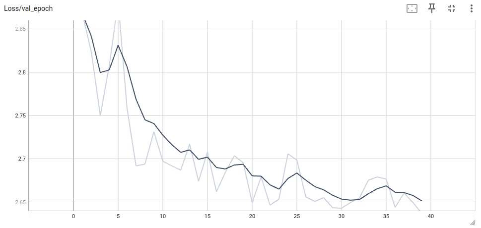
I trained for 40 epochs, which took about 24 hours on a Ryzen 7 3700X CPU, and resulted in roughly one billion 32 ms frames of training data. Below I just show you the skeleton of the training loop, without the tensorboard logging. I also add a screenshot of the validation loss curve from tensorboard, which shows that the model is indeed learning to reconstruct the clean spectrograms from the noisy inputs. The hp variable in the code below houses all the discussed hyperparameters.
def run_quick_val(max_batches: int) -> tuple[float, float]:
    """Run a partial validation pass over *max_batches* batches.

    Temporarily switches the model to eval mode and disables gradient
    computation to save memory, then restores training mode.

    :param max_batches: Maximum number of test batches to evaluate.
    :returns: Tuple of ``(avg_mse_loss, avg_snr_improvement_db)``.
    """
    autoencoder.eval()
    total_loss = 0.0
    total_snr = 0.0
    n_batches = 0

    with torch.no_grad():
        for vinputs, vlabels in test_data:
            if n_batches >= max_batches:
                break
            vinputs = vinputs.float()
            vlabels = vlabels.float()
            voutputs = autoencoder(vinputs)
            total_loss += loss_fn(voutputs, vlabels).item()
            n_batches += 1

    autoencoder.train()
    avg_loss = total_loss / max(n_batches, 1)
    avg_snr = total_snr / max(n_batches, 1)
    return avg_loss, avg_snr

def train_epoch(
    n_iter: int, epoch_number: int, writer: SummaryWriter
) -> tuple[float, int]:
    """Train for one full epoch and return ``(avg_train_loss, n_iter)``."""
    running_loss = 0.0
    recent_loss = 0.0

    for i, (input, label) in enumerate(train_data):
        optimizer.zero_grad()

        prediction = autoencoder(input)
        loss: torch.Tensor = loss_fn(prediction, label)
        loss.backward()
        optimizer.step()

        running_loss += loss.item()
        n_iter += hp.batch_size

        # ── Quick validation every VAL_EVERY batches ──────────────────────────
        if (i + 1) % hp.val_every == 0:
            val_loss, val_snr = run_quick_val(hp.val_batches)

    return recent_loss, n_iter


# Training loop
for epoch in range(hp.n_epochs):
    autoencoder.train()

    avg_loss, n_iter = train_epoch(n_iter, epoch, writer)

    # Full end-of-epoch validation
    epoch_val_loss, epoch_val_snr = run_quick_val(max_batches=10_000)

    # Learning rate scheduling and checkpointing
    scheduler.step(epoch_val_loss)
    current_lr = optimizer.param_groups[0]["lr"]

    if epoch_val_loss < best_val_loss:
        best_val_loss = epoch_val_loss
        model_path = f"{hp.model_dir}/{hp.name}"
        torch.save(autoencoder.state_dict(), model_path)
Results and evaluation
Awesome, we have a trained model! Now, first and foremost, can you test the model? Yes, I built an interactive demo - upload a noisy file, pick a model, and compare the waveforms and spectrograms side by side:
As of now, the Wave-U-Net model in the demo is not trained yet, so don’t expect any performance from it. I will train it in the next part of this series, and update the demo accordingly.
Let me share my observations from testing the model on a variety of noisy speech samples:
- The noise suppression is relatively aggressive, especially at low SNRs, leading to the noise being suppressed so much, that the speech is barely audible.
- The inference time is quite long, especially for longer audio clips, which makes it impractical for real-time applications (you can feel it struggle on my small VPS this runs on). We have to keep in mind that our DAE uses slightly more than two million parameters, which is quite large for a feedforward network. (Compare to Mozillas RNNoise that has just over 80k parameters, and runs in real-time on a CPU at 48 kHz sampling rate).
What remains are some actual numbers for comparing how close we got to the original clean signal, and also how we performed compared to Nossier et al. (2020). I use two metrics for comparison: First, the PESQ (Perceptual Evaluation of Speech Quality) metric, which is a widely used objective measure of speech quality that correlates well with human perception. It asks: “How natural and pleasant does this speech sound compared to the original?”. Second, the STOI (Short-Time Objective Intelligibility) metric, which is an objective measure of speech intelligibility correlating well with human perception. It asks: “Can I actually understand the words being spoken?”. Both metrics are computed using the original clean signal as the reference, and the enhanced signal as the degraded signal.
How exactly these metrics are computed is a bit beyond the scope of this project, but I may cover them in a future post. If you are interested in the details, I recommend reading the original papers by Rix et al. (2001) for PESQ, and Taal et al. (2011) for STOI.
Here is the comparison of our model’s performance with the results reported by Nossier et al. (2020) on the same test set:
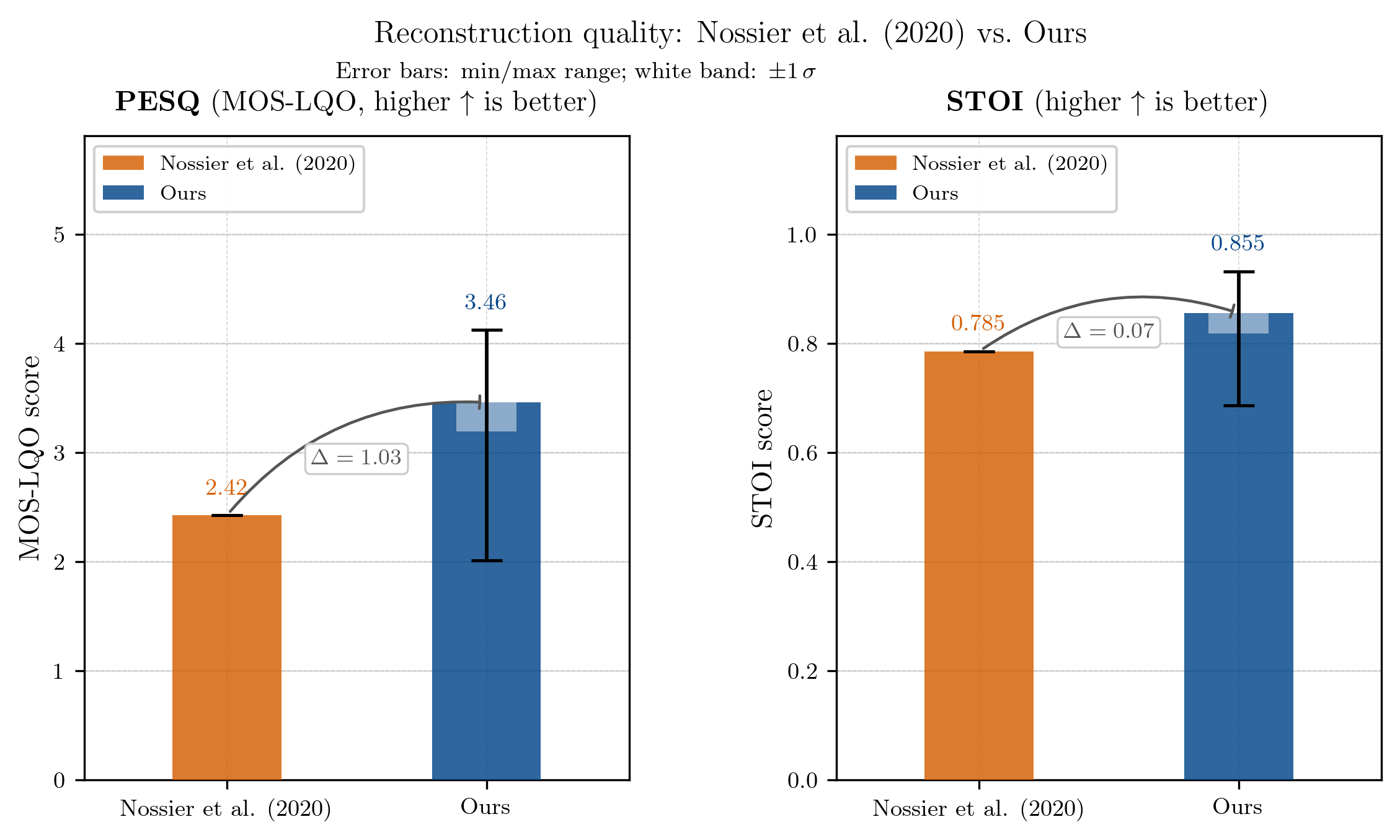
Interestingly, our model outperforms the DAE (d) architecture from Nossier et al. (2020) on both metrics, especially on the PESQ metric, which suggests that our model is able to produce enhanced speech that sounds more natural and pleasant compared to the original noisy signal. I used the entire LibriSpeech test corpus with randomly selected noise at an SNR of 0 dB for this evaluation, which is relatively close to what Nossier did in their paper, but I cannot be sure if the exact same noise segments were used, so the comparison is not entirely fair. However, it is still encouraging to see that our model performs well on these metrics, and it suggests that our implementation of the DAE architecture is effective for speech enhancement tasks.
Outro
Now, that was a lot of ground to cover, but I think we made very good progress in understanding how (somewhat) modern speech enhancement systems work, and we also got to implement a DAE from scratch, which is pretty cool.
In the next and final part of this series, we will explore a more advanced architecture for speech enhancement, which is based on the U-Net architecture that was originally proposed for image segmentation tasks. Stay tuned for that, and in the meantime, feel free to check out the code and the demo, and let me know if you have any questions or feedback!
Literature
Jannu, Chaitanya, and Sunny Dayal Vanambathina. “An overview of speech enhancement based on deep learning techniques.” International Journal of Image and Graphics 25.01 (2025): 2550001.
Nossier, Soha A., et al. “An experimental analysis of deep learning architectures for supervised speech enhancement.” Electronics 10.1 (2020): 17.
Panayotov, Vassil, et al. “Librispeech: an asr corpus based on public domain audio books.” 2015 IEEE international conference on acoustics, speech and signal processing (ICASSP). IEEE, 2015.
Pascual, Santiago, Antonio Bonafonte, and Joan Serra. “SEGAN: Speech enhancement generative adversarial network.” arXiv preprint arXiv:1703.09452 (2017).
Rix, Antony W., et al. “Perceptual evaluation of speech quality (PESQ)-a new method for speech quality assessment of telephone networks and codecs.” 2001 IEEE international conference on acoustics, speech, and signal processing. Proceedings (Cat. No. 01CH37221). Vol. 2. IEEE, 2001.
Rumelhart, David E., Geoffrey E. Hinton, and Ronald J. Williams. “Learning representations by back-propagating errors.” nature 323.6088 (1986): 533-536.
Stoller, Daniel, Sebastian Ewert, and Simon Dixon. “Wave-u-net: A multi-scale neural network for end-to-end audio source separation.” arXiv preprint arXiv:1806.03185 (2018).
Taal, Cees H., et al. “An algorithm for intelligibility prediction of time–frequency weighted noisy speech.” IEEE Transactions on audio, speech, and language processing 19.7 (2011): 2125-2136.
Thiemann, Joachim, Nobutaka Ito, and Emmanuel Vincent. “The diverse environments multi-channel acoustic noise database (demand): A database of multichannel environmental noise recordings.” Proceedings of Meetings on Acoustics. Vol. 19. No. 1. Acoustical Society of America, 2013.
Valin, Jean-Marc. “A hybrid DSP/deep learning approach to real-time full-band speech enhancement.” 2018 IEEE 20th international workshop on multimedia signal processing (MMSP). IEEE, 2018.
Vincent, Pascal, et al. “Extracting and composing robust features with denoising autoencoders.” Proceedings of the 25th international conference on Machine learning, 2008.