Speech Enhancement using Deep Learning 2/? - Further Concepts

Goal and rationale

In the previous post on this project, we did some heavy lifting to motivate and understand the ingenious Discrete Fourier Transform (DFT), to show that we can decompose a time-domain signal into its frequency components by making use of some clever math. In this sequel, I want to extend our understanding of the DFT by introducing some concepts that are crucial for understanding how to use it in practice, including spectral leakage, windowing, the Short-Time Fourier Transform (STFT), and - of course - the inverse DFT.

Analysis frequencies

Let’s recall the DFT formula from the last post. For a real-valued, discrete signal $x_n$ of length $N$, the DFT is defined as

$$X_k = \sum_{n=0}^{N-1} x_n e^{-2\pi i\tfrac{n}{N}k} \quad \text{for } k = 0, 1, \ldots, N-1.$$

In the previous post, we showed that the DFT is able to decompose the signal $x_n$ into its frequency components, by analyzing how much of a certain frequency $k$ is in our signal. Crucially, $k$ is given is cycles / signal-duration, or

$$k \mathrel{\widehat{=}} \frac{k}{T}[Hz],$$

where $T$ is the duration of the signal in seconds. To give an example, we can look at the signal from our previous post, which had a length of exactly 1 second. Therefore, all $k$-values correspond neatly to the integer $\frac{k}{1}Hz$ equivalents.

In general, all frequencies

$$\frac{k}{T}[Hz], \quad \text{for } k= 1 \dots N-1$$

are called our analysis frequencies, as they represent the frequencies we can unequivocally identify from our signal, of course only up to the Nyquist frequency, otherwise aliasing occurs.

If we look back at our magnitude plot, we observe that we have a neat peak at exactly $2 Hz$, while it being zero everywhere else. From what we learned this makes sense, as one of the analysis frequencies of our DFT exactly matches the frequency of our signal ($k=2 \rightarrow 2 \, Hz$).

But what happens if this is not the case?

Spectral leakage

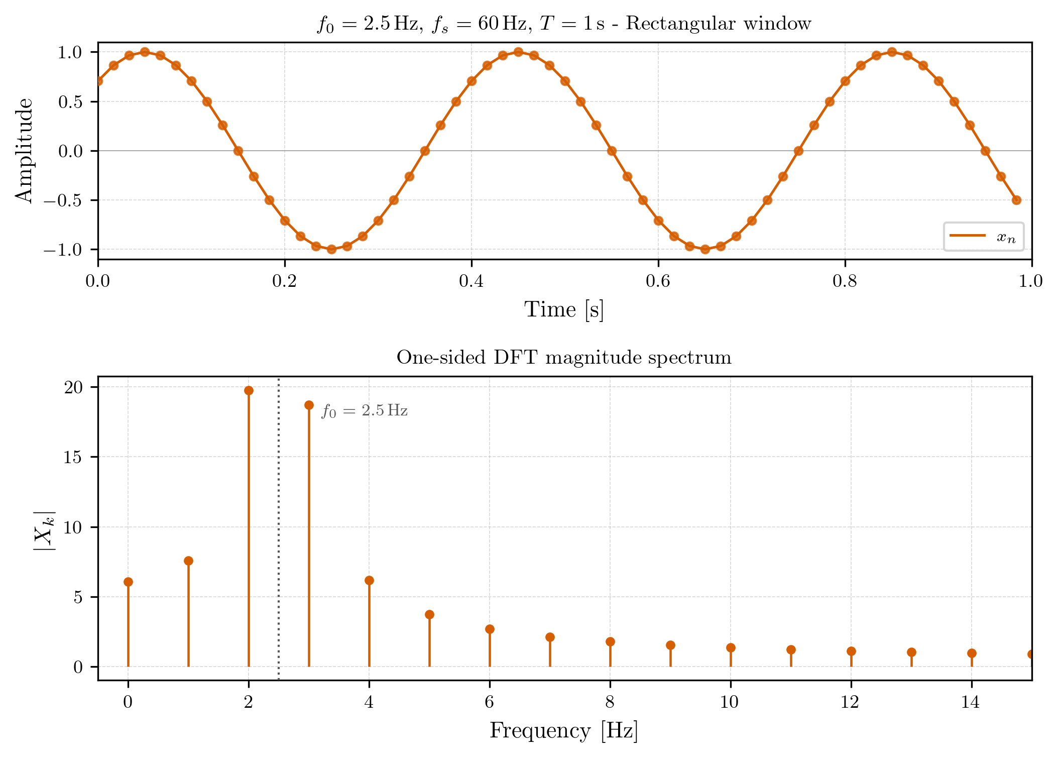
Consider the following two signals, of which one is our original $2 \, Hz$ signal (blue), and the other is a $2.5 \, Hz$ signal (orange). They are both sampled at $60 \, Hz$ for $1 \, s$:

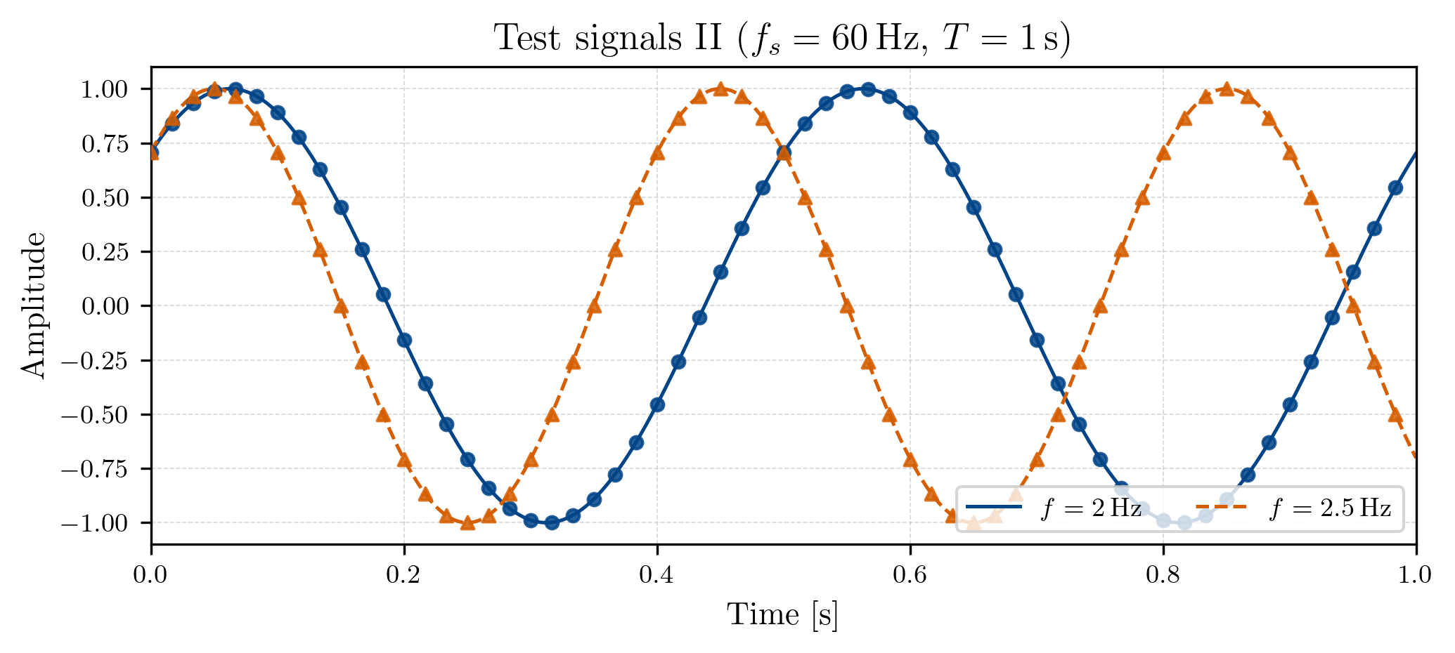
From this image and what we figured out so far, we can make two crucial observations.

1. $2.5 \, Hz$ is not an analysis frequency of our DFT ($\nexists k \in \mathbb{Z}: k = 2.5$) which are given by integer multiples of $\frac{k}{T}=\frac{k}{1}[Hz]$ for $k = 0, 1, \dots, 59$.

2. The $2.5 \, Hz$ signal does not complete an integer number of cycles within the 1 second duration of our signal, while the $2 \, Hz$ signal does.

In fact, both of these observations are just two different ways of saying the same thing. If a signal completes an integer number of cycles within the duration of our signal, then it will always be an analysis frequency of our DFT (again, which we can only sensibly identify up to the Nyquist frequency), and vice versa.

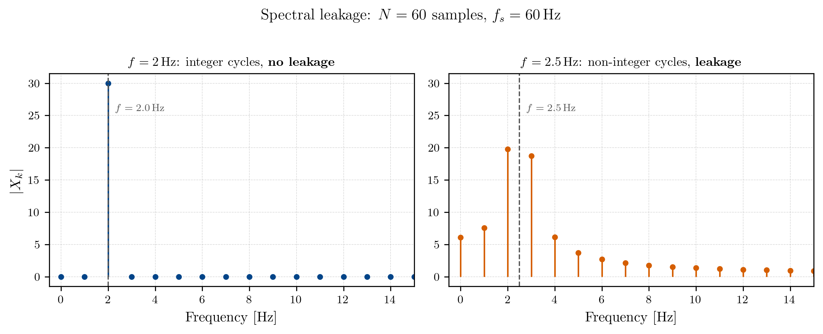
We will now see that if a signal does not complete an integer number of cycles within the duration of our signal, the energy of that signal will “smear” across all frequencies in the DFT, instead of being concentrated at a single frequency bin. This phenomenon is called spectral leakage and looks like this in the spectrum:

Why exactly this happens is relatively straightforward to show, but involves a bit of math. If you just want to know what we can do to avoid or at least mitigate spectral leakage, you can skip the next part and jump to the section on windowing.

Spectral leakage as a consequence of the DFT’s implicit rectangular window

One way to understand spectral leakage is to imagine our signal as a cut-out of an infinite, continuous signal. Therefore, let $x(t)$ be our (continuous) signal, $w(t)$ the “cut-out function”, which in signal processing usually is called the window function. To get the cut-out signal we want, our window function has to be the rectangle function, that has a value of 1 where our target part of the signal is, and 0 everywhere else. In gneneral, the rectangle function is defined as:

$$w(t) = \text{rect}\left(t\right) = \begin{cases} 0 & \text{if } |t| \geq \frac{1}{2} \\ 1 & \text{if } |t| \leq \frac{1}{2} \end{cases}.$$

The idea of our proof, revolves around the convolution theorem of the Fourier analysis, stating that the Fourier transform of a product of two functions is equal to the convolution of their Fourier transforms. Formally,

$$\mathcal{F}\{x(t) \cdot w(t)\} = X(f) * W(f),$$

where $\mathcal{F}$ is the Fourier transform, $X(f)$ and $W(f)$ are the Fourier transforms of $x(t)$ and $w(t)$ respectively, and $*$ is the convolution operator. A consequence of this is, that multiplication of two functions in the time domain corresponds to convolution of their Fourier transforms in the frequency domain:

$$x(t) \cdot w(t) \rightleftharpoons X(f) * W(f).$$

Now, what we hope to prove here is, that when we convolve the transform of our $2.5 \, Hz$ signal with the transform of the rectangular window function, we will be able to see how the spectral leakage arises out of it. Great, so let’s make plan:

1. Calculate the Fourier transform of our $2.5 \, Hz$ signal
2. Calculate the Fourier transform of the rectangular window function
3. Convolve the two, and see how this affects our spectrum

First, we define our signal, and also convert it to complex exponential form to ease later calculation.

$$x(t) = \sin(2\pi f_0 t) = \frac{1}{2i}(e^{i 2\pi f_0 t} - e^{-i 2\pi f_0 t}),$$

where $f_0$ will be the $2.5 \, Hz$ in our example. The standard definition of the continuous-time (we will go back to discrete-time very soon) Fourier transform is

$$X(f) = \int_{-\infty}^\infty x(t) e^{-2\pi i f t} \mathrm{d}t.$$

Replacing $x(t)$ with our signal and integrating gives us

$$\begin{aligned} X(f) &= \int_{-\infty}^\infty \left[\frac{1}{2i}(e^{2\pi i f_0 t} - e^{-2\pi i f_0 t})\right] e^{-2\pi i f t} \mathrm{d}t.\\ &= \frac{1}{2i} \int_{-\infty}^\infty e^{2\pi i f_0 t} e^{-2\pi i f t} \mathrm{d}t - \frac{1}{2i} \int_{-\infty}^\infty e^{-2\pi i f_0 t} e^{-2\pi i f t} \mathrm{d}t. && \text{linearity}\\ &= \frac{1}{2i} \int_{-\infty}^\infty e^{2\pi i (f_0 - f) t} \mathrm{d}t - \frac{1}{2i} \int_{-\infty}^\infty e^{-2\pi i (f_0 + f) t} \mathrm{d}t. \end{aligned}\tag{1}$$

Given the definition of the Dirac delta function

$$\delta(\nu) = \int_{-\infty}^\infty e^{2\pi i \nu t} \mathrm{d}t,$$

we can replace the integrals in (1) with delta functions, by setting $\nu = f_0 - f$ in the first part and $\nu = f_0 + f$ in the second part, which gives us

$$\begin{aligned} X(f) &= \frac{1}{2i} \delta(f_0 - f) - \frac{1}{2i} \delta(f_0 + f) \\ &= \frac{1}{2i} \delta(f - f_0) - \frac{1}{2i} \delta(f + f_0). && \text{symmetry of delta function} \end{aligned}$$

For our $2.5 \, Hz$ signal,

$$X(f) = \frac{1}{2i} \delta(f - 2.5) - \frac{1}{2i} \delta(f + 2.5),$$

meaning that all the energy of our signal is concentrated at $2.5 \, Hz$ and $-2.5 \, Hz$ (the negative frequency component is just a mathematical artifact of our complex exponential representation of the signal, and does not have a physical meaning in our case).

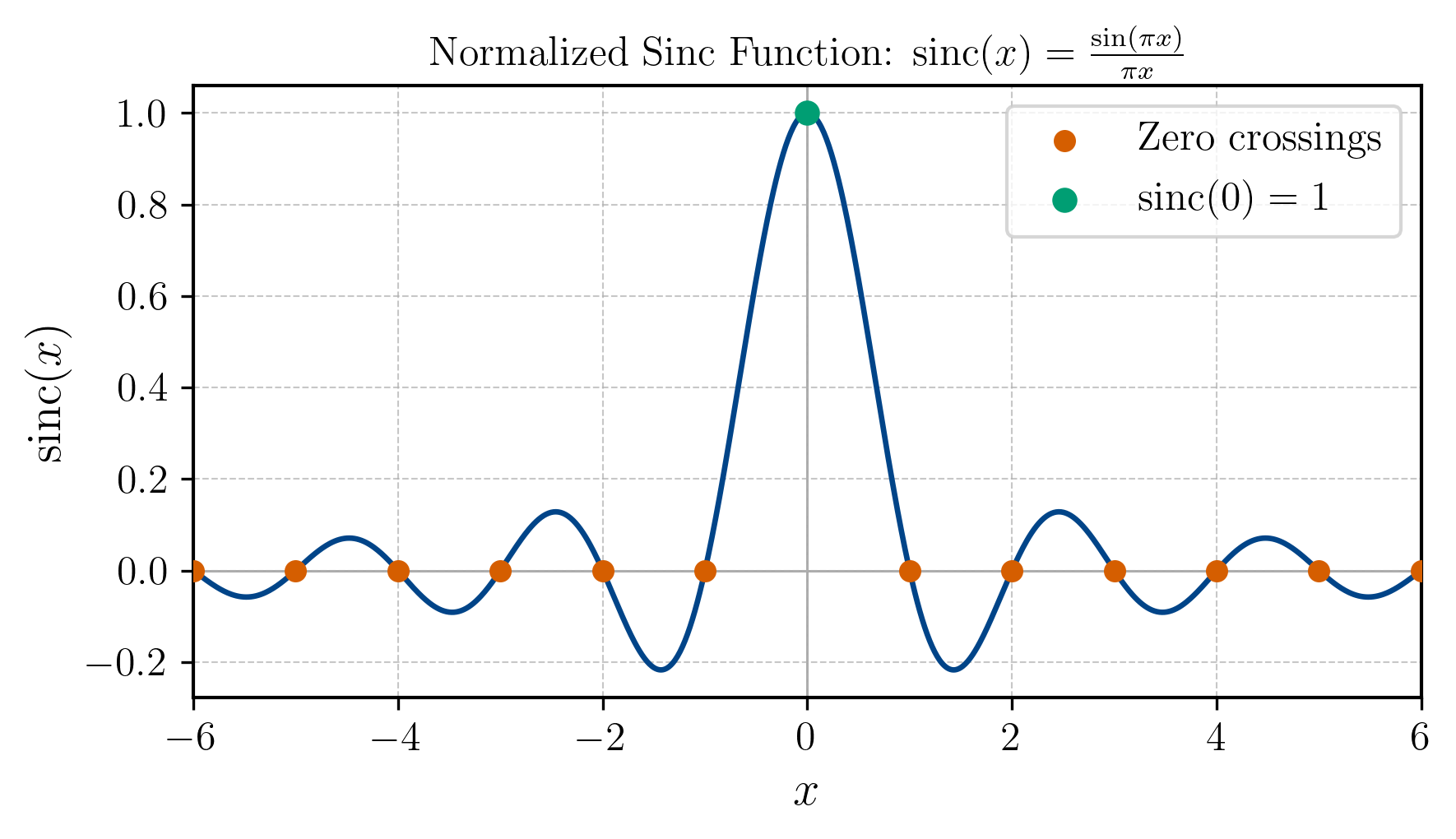
For the rectangular window function, we can calculate its Fourier transform as follows:

$$\begin{aligned} W(f) &= \int_{-\infty}^\infty w(t) \cdot e^{-2\pi i f t} \mathrm{d}t \\ &= \int_{-\infty}^\infty \text{rect}(t) \cdot e^{-2\pi i f t} \mathrm{d}t \\ &= \int_{-\frac{1}{2}}^{\frac{1}{2}} (1) \cdot e^{-2\pi i f t} \mathrm{d}t && \text{definition of rectangular window}\\ &= \left[ \frac{e^{-2\pi i f t}}{-2\pi i f} \right]_{-\frac{1}{2}}^{\frac{1}{2}} && \text{integration}\\ &= \frac{1}{2\pi i f} \left(e^{\pi i f} - e^{-\pi i f}\right) \\ &= \frac{1}{\pi f} \sin(\pi f) && \text{Euler's formula}\\ &= \text{sinc}(f) && \text{def. normalized sinc function} \end{aligned}$$

As we can see, the Fourier transform of the rectangular window function is the normalized sinc function which looks like this:

The only thing left to do now, is to convolve $X(f)$ with $W(f)$. The formal definition of convolution is

$$(X * W)(f) = \int_{-\infty}^\infty X(\tau) W(f - \tau) \mathrm{d}\tau.$$

For our case, let us only look at the positive frequency part of $X(f)$, as the negative frequency part is just a mirror image of it.

$$\begin{aligned} (X * W)(f) &= \int_{-\infty}^\infty \left[\frac{1}{2i} \delta(\tau - 2.5)\right] W(f - \tau) \mathrm{d}\tau \\ &= \frac{1}{2i} \int_{-\infty}^\infty \delta(\tau - 2.5) W(f - \tau) \mathrm{d}\tau \\ &= \frac{1}{2i} W(f - 2.5) && \text{sampling property of delta function}\\ &= \frac{1}{2i} \text{sinc}(f - 2.5). \end{aligned}$$

The sampling property of the delta function arises from the fact that the delta function is zero everywhere except at the point where its argument is zero, where it is infinite, while its integral over the entire real line still is equal to 1. Therefore, when we integrate a function multiplied by a delta function, we are essentially “sampling”, or “pulling out” the function value at the point where the delta function is non-zero.

The only thing left to do now, is to look at the magnitude of our spectrum, which is given by

$$|X * W|(f) = \left|\frac{1}{2i} \text{sinc}(f - 2.5)\right| = \frac{1}{2} |\text{sinc}(f - 2.5)|.$$

Okay, that was a lot of math, so let us take a step back and remind ourselves of the bigger picture. All we wanted was to show, why a signal that does not complete an integer number of cycles within the duration of our signal, has a smeared spectrum across all frequencies, while a signal that does complete an integer number of cycles has a neat peak at its frequency. If you perform the same convolution for the $2 \, Hz$ signal, we will see that its spectrum is the same sinc function, but centered at $2 \, Hz$ instead of $2.5 \, Hz$.

Let’s plot both of these spectra together (and drop the constant $\frac{1}{2}$ of the sinc for better visualization):

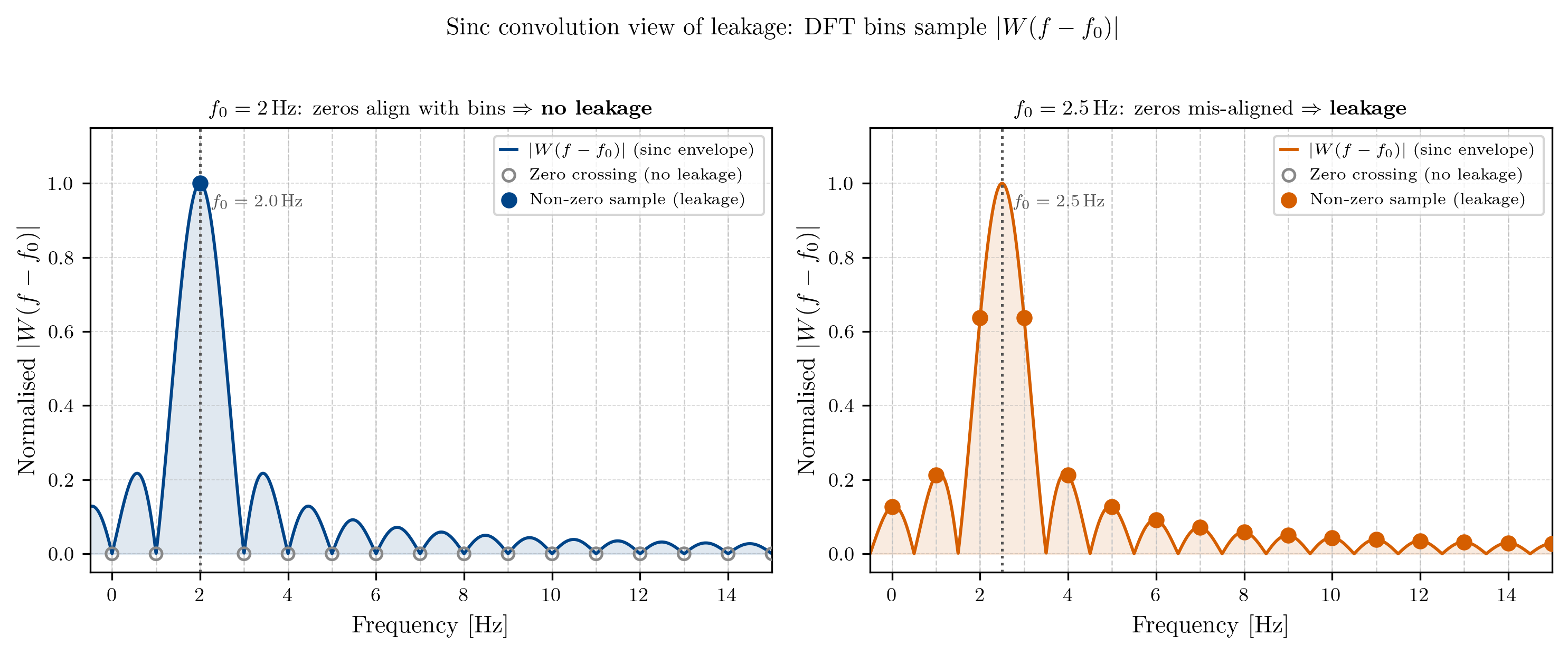
Now, here is the crucial part. In our discrete case, we only have access to the values of the spectrum at the analysis frequencies, which are given by integer multiples of $\frac{k}{T}$, or in our example at integer frequencies. Further, for the sinc function it holds that $\text{sinc}(x)= 0 \quad \forall x\in \{n \ \mid \ n\in \mathbb {Z} \setminus \{0\}\}$. In the figure above, we can see that for our $2 \, Hz$ signal, all analysis frequencies except for $2 \, Hz$ are located at the zero-crossings of the sinc function, meaning that we will only see a peak at $2 \, Hz$ in our spectrum. For our $2.5 \, Hz$ signal however, all analysis frequencies are located at points where the sinc function has non-zero values, meaning that we will see energy at all frequencies in our spectrum, which is exactly what we observed in Fig. 2 $\blacksquare$.

Windowing

Obviously, spectral leakage is not a desirable phenomenon, and to make matters worse, it cannot be avoided in general, as “the energy in a signal associated with each frequency has to go somewhere in the DFT, and if the frequency does not correspond to one of our analysis frequencies, then it will spread out.” - Brian McFee.

The good news is, that we can control the magnitude of the leakage by a technique called windowing.

In the previous section, we showed that the leakage mathematically arises, because our signal has to be interpreted as a finite-time cut-out of an infinite signal. To arrive at a signal that that is zero everywhere, except where we observe it, we set the “cut-out function” $w(t)$ to be the rectangle function that is 1 where our target part of the signal is, and 0 everywhere else. However, exactly the choice of $w(t)=\text{rect}(t)$ causes all of the leakage.

The general idea is, to multiply our signal by a different window function than the rectangle, such that we force all frequencies to perform an integer amount of cycles. The standard way to do this is to force the signal to smoothly approach $x_0 \approx x_{N-1} \approx 0$. This results in a windowed DFT $\hat{X}$:

$$\hat{X} = \mathcal{F}\{x_n \cdot w_n\},$$

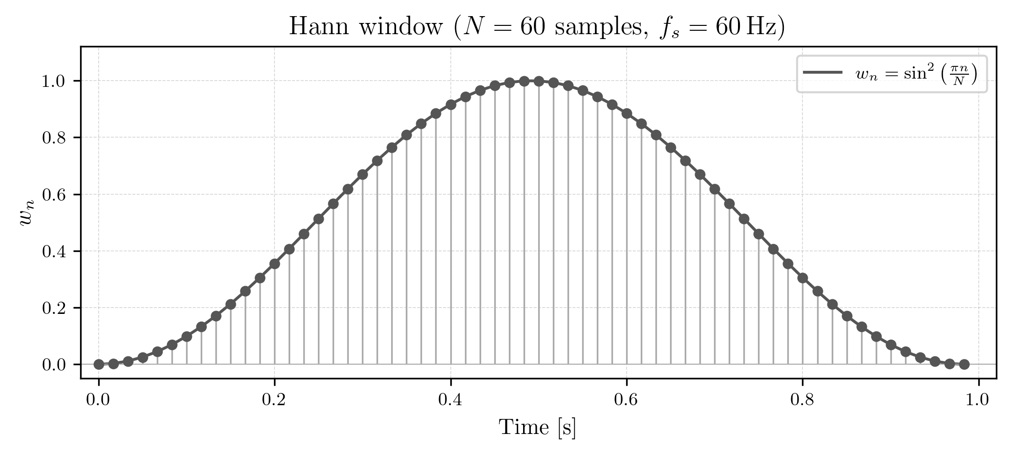
where $w_n$ is a discrete window function. A very common choice for $w_n$ is the Hann window, which is defined as

$$w_n = \sin^2\left(\frac{\pi n}{N}\right), \quad \text{for } 0 \leq n \leq N-1,$$

and for our example looks like this:

If we now were to apply the Fourier transform to our signal after applying the Hann window, we can observe that the spectral leakage is significantly reduced, as the energy of our signal is now more concentrated around its true frequency,

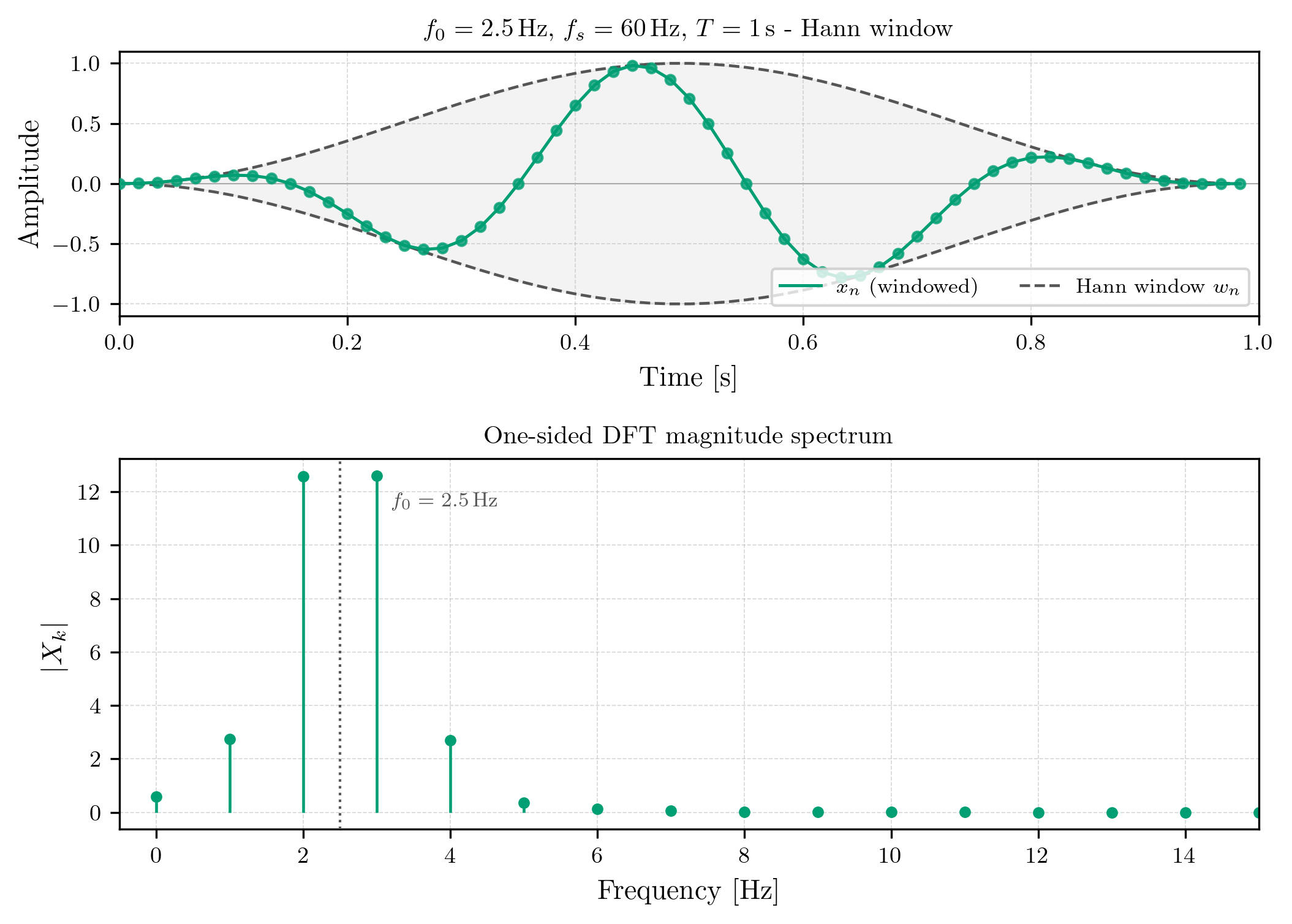
compared to the rectangular window case:

The Hann window is just one of many different proposed window functions. You can find a longer list of functions on the Wikipedia and a more detailed discussion of their properties in McFee’s chapter on it.

In conclusion:

1. Spectral leakage is an inherent, and unavoidable phenomenon of the DFT, arising from the fact that we are analyzing a finite-time, cut-out of an infinite signal, using an implicit rectangular window function. In case this cut-out does not contain an integer number of cycles of a certain frequency, the energy of that frequency will be smeared across all frequencies in the DFT, instead of being concentrated at a single frequency bin.

2. We can control the magnitude of the leakage by applying a window function, different from the implicit rectangular window, to our signal before applying the DFT. There exist many different window functions, but the Hann window is a general-purpose-choice for many signal processing applications.

The Short-Time Fourier Transform (STFT)

The techniques we have discussed so far, allow us to transform a signal from the time domain to the frequency domain, where we can inspect the magitudes of the frequencies building our signal. What our current knowledge does not allow us to do, however, is to see how the frequencies of a signal change with time. If we remember the footsteps signal from the first part, we would expect there to be lower and louder frequencies when the foot touches the floor, and higher and more quiet ones when the foot is moving. To do this, we use the concept of the STFT, and it’s straight forward to grasp.

In principle the STFT does nothing more than to apply the DFT to small chunks of our signal, so that we get a spectrum for each one. We can then view these resulting spectra over time, to actually see our frequencies evolve. Formally:

$$\mathbf {STFT}_k \{x_n\}(m)\equiv X_k(m)=\sum _{n=0 }^{L-1}x_{[n+mH]} w_{n}e^{-2 \pi i \frac{n}{N}k},\\ \text{for } m = 0, 1, \dots, M-1 \text{ and } k = 0, 1, \dots, N-1.$$

Here, $w_n$ is a window function, which we apply to each chunk of our signal, to mitigate spectral leakage. The parameter $H$ is the hop size, which determines how much we shift our window for each chunk. $L$ is the window length, and $M$ is the number of chunks. For example, if we have a signal of length 1000, and we choose $L=100$ and $H=50$, we will get spectra for the following chunks of our signal: $x_0 \dots x_{99}$, $x_{50} \dots x_{149}$, $x_{100} \dots x_{199}$, and so on.

The formula may look a bit intimidating at first, but it is really just a straightforward extension of the DFT formula we already know, with the addition of the window function and the hop size. The resulting STFT is a 2D matrix, where each column corresponds to the spectrum of a chunk of our signal, and each row corresponds to a frequency bin. We can visualize this matrix as a spectrogram, which is a heatmap of the magnitudes of the frequencies over time.

Let’s look at an example of a spectrogram of our footstep signal. Let’s go with some arbitrary parameters. We will use a window length of $L=1024$ samples, a hop size of $H=512$ samples, and a Hann window:

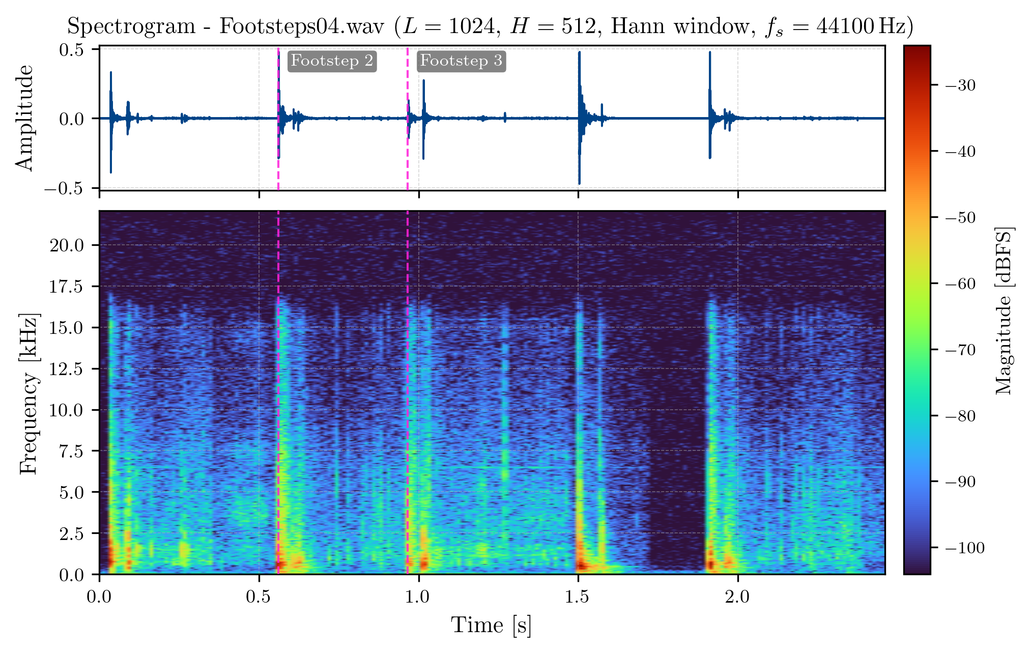
The bottom part of the figure above shows the spectrogram of our footstep signal, with the magnitues in full-scale decibels $dBFS= 20 \log_{10} \left(|X_k(m)|\right)$. We read this spectrum relatively intuitively as follows: the x-axis corresponds to time, and the y-axis corresponds to frequency. The color of each point in the spectrogram corresponds to the magnitude of that frequency at that time, with brighter colors indicating higher magnitudes. The two vertical lines in the spectrogram correspond to two selected footstep events. As proposed earlier, we can indeed see that there are higher and more quiet frequencies when the foot is moving, and lower and louder frequencies when the foot touches the floor.

As with every topic we discuss in this series, there is a lot more to say about the STFT, but one concept in particular I want to cover, as it fundametally limits how accurate the STFT can get: the Gabor Limit.

The Gabor Limit is basically the uncertainty principle of signal processing, stating that there is a trade-off between the time resolution and the frequency resolution of the STFT. In other words, if we want to have a high time resolution (i.e., be able to see how frequencies change very quickly), we have to use a short window length $L$, which will result in a low frequency resolution (i.e., we won’t be able to distinguish between closely spaced frequencies). Conversely, if we want to have a high frequency resolution, we have to use a long window length, which will result in a low time resolution. We can easily show this with an example. Consider a signal that is sampled at $1000 \, Hz$ and has a duration of $1 \, s$. If we choose a window length of $L=1000$ samples, we will get a frequency resolution of $\frac{1000}{1000} = 1 \, Hz$, meaning that we can distinguish between frequencies that are at least $1 \, Hz$ apart. However, if we choose a window length of $L=100$ samples, we will get a frequency resolution of $\frac{1000}{100} = 10 \, Hz$, meaning that we can only distinguish between frequencies that are at least $10 \, Hz$ apart. This trade-off is a fundamental limitation of the STFT, and it is important to keep it in mind when choosing the parameters for our speech enhancement model later.

The Inverse DFT

So far, we have only been moving from the time domain into the frequency domain. The Inverse DFT (IDFT) does exactly the opposite: given a spectrum $X_k$, it reconstructs the original time-domain signal $x_n$. The intuition is simple - instead of decomposing a signal into complex sinusoids by projecting onto them, we sum those sinusoids back up, each weighted by its corresponding frequency-domain coefficient:

$$x_n = \frac{1}{N} \sum_{k=0}^{N-1} X_k \, e^{2\pi i \frac{n}{N}k}, \quad n = 0, 1, \dots, N-1.$$

Comparing this with the DFT formula, the only differences are the sign in the exponent (now positive) and the normalization factor $\frac{1}{N}$. Together, these two operations form a perfect pair: apply the DFT to go to the frequency domain, manipulate the spectrum as desired, then apply the IDFT to return to the time domain. This round-trip property makes the IDFT the essential ingredient in any speech enhancement pipeline: after we have estimated which parts of the spectrum belong to noise, we can suppress them and reconstruct a clean signal.

Summary

In this post, we extended our understanding of the DFT with four key concepts that are essential for applying it in practice:

1. Analysis frequencies: the DFT does not give us a continuous spectrum, but rather evaluates it at a discrete set of frequencies $\frac{k}{T}$ for $k = 0, 1, \dots, N-1$. Only signals whose frequency coincides with one of these analysis frequencies are represented cleanly.

2. Spectral leakage: when a signal does not complete an integer number of cycles within the observation window, its energy smears across all frequency bins. This is an inherent consequence of implicitly multiplying the signal by a rectangular window, whose Fourier transform is the sinc function. Convolution of the signal’s spectrum with this sinc function is what produces the leakage.

3. Windowing: by replacing the implicit rectangular window with a smoother alternative (such as the Hann window), we can force the signal to taper smoothly to zero at both ends. This significantly reduces the magnitude of the leakage, at the cost of a slightly wider main lobe.

4. The STFT: to track how frequencies evolve over time, we slide a window across the signal and apply the DFT to each overlapping chunk. The result is a 2D time-frequency representation called a spectrogram. The Gabor Limit tells us that there is an unavoidable trade-off between time resolution and frequency resolution: a shorter window gives better time resolution but coarser frequency bins, and vice versa.

5. The Inverse DFT: the IDFT inverts the DFT by summing the complex sinusoids back up, each weighted by its spectral coefficient. Together, the DFT and IDFT form a lossless round-trip between the time and frequency domains, which is the cornerstone of the speech enhancement workflow we will build in the next posts.

Perfect! In the next post, we will finally start building our first model, the “denoising autoencoder”, where all the concepts we have covered so far and even more will come together in a beautiful way. See you in the next one!

---

Literature

McFee, Brian. Digital Signals Theory. Chapman and Hall/CRC, 2023.