Speech Enhancement using Deep Learning 1/? - The DFT

Goal and rationale

I was chatting with my wife the other day and asked if she’d left the office yet. “On my way to the tram”, she responded, which got me confused: there wasn’t any background noise on her end. When she confirmed she was indeed outside on the sidewalk, I realized just how impressive her phone’s noise suppression must be. It got me wondering: how does that technology actually work, and could I implement something similar myself?

This blog post is the first in a series where I’ll be exploring various deep learning approaches to speech enhancement. The idea is to take audio recordings of speech that are contaminated with noise and train a neural network to produce cleaner versions of those recordings. Along the way, I’ll be revisiting some fundamental concepts in digital signal processing (DSP) and machine learning, to make sure we have a solid foundation before diving into the implementation.

The journey will, hopefully, cover some ground on older deep learning approaches like autoencoders, as well as more recent transformer-based architectures. I will also be exploring different input representations for our models, such as spectrograms and raw waveforms, and discussing the trade-offs between them.

Here, I want to highlight the book “Digital Signals Theory” by Brian McFee (who is also one of the authors of the librosa library). Reading it provides a very hands-on, yet deep introduction into most of the foundational concepts we will be touching here. You can access it online here.

But let’s not get ahead of ourselves. Since this is also my first touching point with digital signal processing, I want to start with the basics and build up our understanding from there. In this first post, I will be focusing on the Discrete Fourier Transform, which is a fundamental tool in DSP and is widely used in audio processing tasks, including speech enhancement.

Motivating the Discrete Fourier Transform (DFT)

Whenever we talk about processing audio signals, the DFT is bound to come up. Since it is arguably one of the most important transforms, maybe ever, a solid understanding of it is crucial for our project. Also, the DFT is such an ingenious mathematical tool that it’s worth revisiting just for the sake of appreciating its beauty.

There is an entire field of mathematics called Fourier analysis dedicated to studying the properties and applications of the Fourier transform, of which the DFT is a discrete version. Therefore, it’s impossible to cover all the details in a single blog post. Instead, I will focus on the aspects of the DFT that are most relevant to our speech enhancement project, and using the DFT for audio processing in general.

Imagine you recorded a person walking down a hallway with a microphone. In doing so, the microphone captures the displacement of its membrane over time, and translates them into voltage readings. If we were to plot these voltage readings against time, we would see a waveform that represents the sound of the footsteps. You can see an example of such a waveform in the figure below:

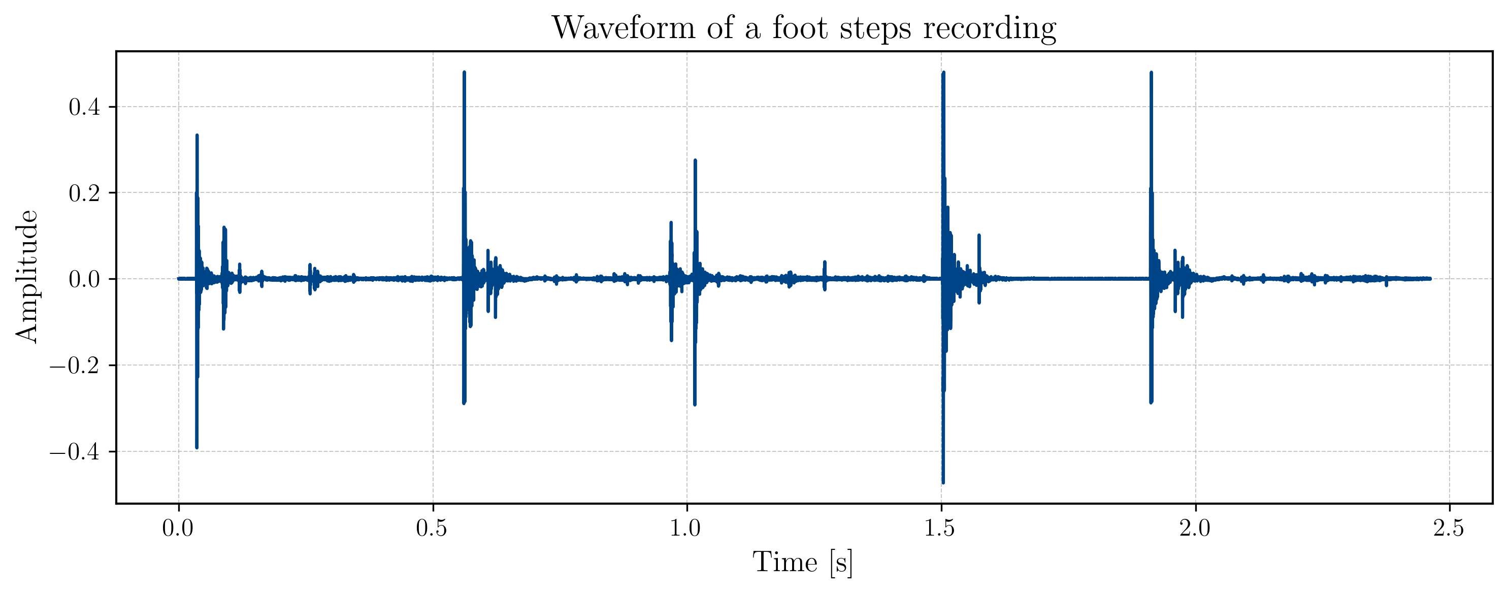
You can listen to the audio recording of the footsteps too:

Now, while showing us information on how our signal evolves over time, the waveform does not tell us much about the frequencies that are present in the signal. For our speech enhancement task, however, it would be of great interest to know which frequencies we are dealing with. As an adjacient example, one could imagine that you make a phone call while staning next to a humming air conditioner. The noise from the air conditioner might be concentrated in a specific frequency range, and if we could identify that range, we could potentially filter it out to improve the quality of the phone call. This is where the DFT comes in. The DFT allows us to transform our time-domain signal into the frequency domain, where we can analyze the different frequency components that make up our signal.

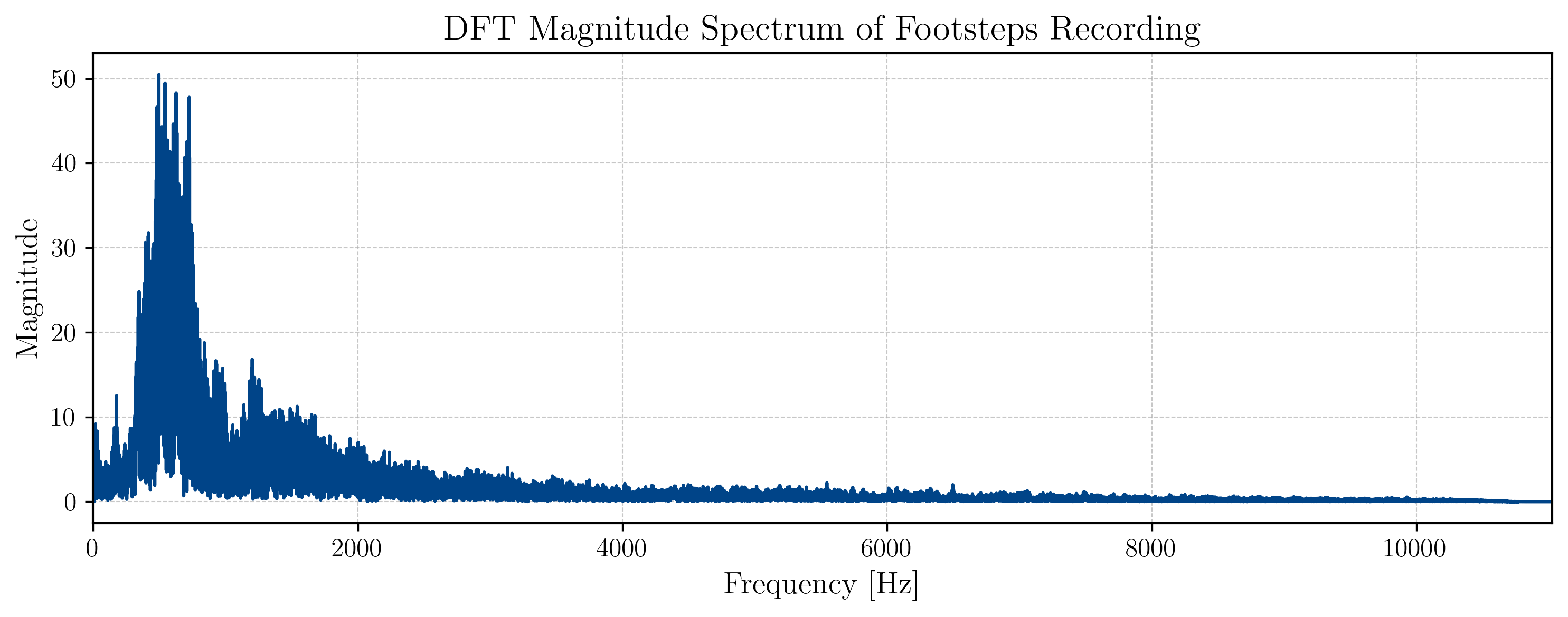
Our goal will be to arrive at a representation of our signal that looks something like this:

Defining and understanding the DFT

The way I want to present the DFT is by first giving you its definition, and then calculating it for a simple example signal to showcase its inner workings. During this process, I will also cover some of the its properties and implications, and how it relates to our speech enhancement project.

Essentially, the DFT transforms a sequence of $N$ real or complex numbers $\{\boldsymbol{x}_n\} := x_0, x_1, \dots, x_{N-1}$ into another sequence of $N$ complex numbers $\{\boldsymbol{X}_k\} := X_0, X_1, \dots, X_{N-1}$ according to the following formula:

$$X_k = \sum_{n=0}^{N-1} x_n e^{-i 2\pi k n / N}.\tag{1}$$

In operator notation, this is often written as

$$\mathbf{X} = \mathcal{F} \{\mathbf{x}\}.$$

How exactly this translates into a transformation from the time domain to the frequency domain will become clear once we work through an example. As many others, I will use the “winding machine” analogy to explain how frequencies emerge as a result from the DFT (in case you missed it, 3Blue1Brown’s video on the Fourier transform is highly recommended). Additionally, I will also show a full calculation of the DFT for a simple signal, to prove that the intuition we are building with the winding machine analogy is actually correct.

The signal we will be working with in the example is a 1 second long simple 2 Hz sine wave (phase-shifted by $\pi/4$) sampled at 6 Hz (the sampling rate $f_s$), which gives us the following sequence of 6 samples, each colored differently for better visualization:

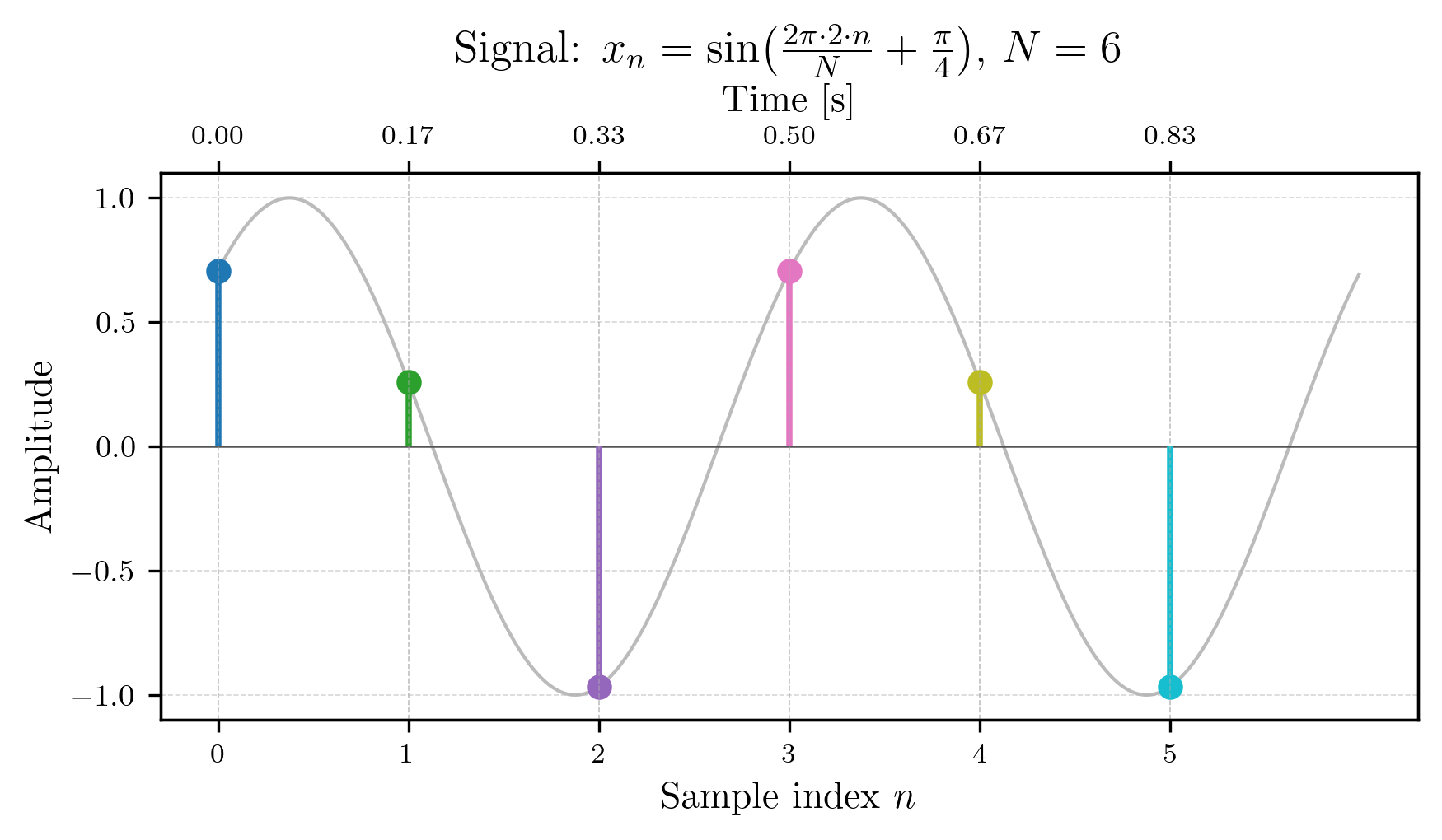
Just for clarifictation, the grey signal in the figure above is the original continuous-time sine wave (the truth we don’t know), while the colored dots represent the discrete samples that you would obtain if you were to measure the signal at 6 equidistant points in time over the course of 1 second. The sample values are as follows:

$$\{\boldsymbol{x}_n\}=[0.707, 0.259, -0.966, 0.707, 0.259, -0.966]$$

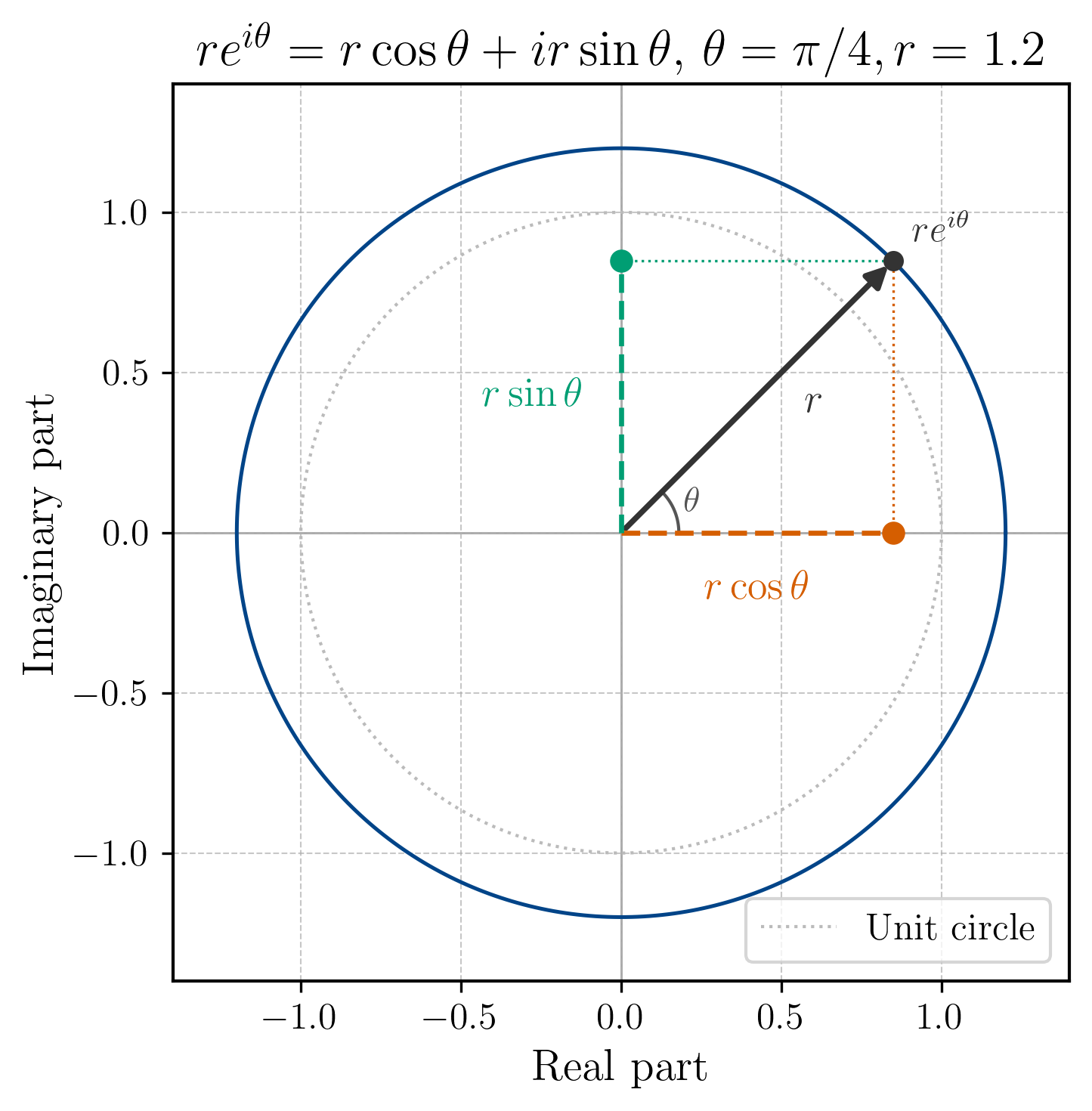
The winding machine

For the winding machine analogy, we remember that a complex number can be represented in polar form $r e^{i\theta}$, where $r$ is the magnitude and $\theta$ is the angle. Specifically, $e^{i\theta}$ encodes a counter-clockwise rotation of angle $\theta$ from the positive real axis. The figure below provides a visual recap of this concept (together with the decomposition of the complex exponent into its sine and cosine components):

For our DFT we have $\theta = -2\pi i\frac{n}{N}k$. This tells us two things: first, that due to the negative sign, we have a clockwise rotation; and second, that the magnitude rotation we impose on our signal depends on our choice of $k$. In fact, for each value of $k$, we have a different rotation pattern that we apply to our signal.

If we look back to the definition in (1), we can now understand how frequencies can emerge from the DFT procedure. The value $k$ determines how many times we rotate our signal around the unit circle as we sum over $n$. For example, if $k=1$, we have a rotation of $-2\pi i\frac{n}{N}$, which means that as $n$ goes from 0 to $N-1$, we will complete one full clockwise rotation around the unit circle. If $k=2$, we will complete two full rotations, and so on.

Critical insight: If we now know the sampling rate $f_s$ of our signal, i.e. the number of samples per second, we can determine the frequency associated with each value of $k$. Specifically, the frequency corresponding to $k$ is given by:

$$f_k = \frac{k}{N} \cdot f_s$$

Just as a sanity check, we can verify that for our example signal, which is a 2 Hz, 1 second sine wave sampled at 6 Hz, for $k=2$ we have:

$$f_2 = \frac{2}{6} \cdot 6 \text{ Hz} = 2 \text{ Hz}$$

which means that the DFT component corresponding to $k=2$ (i.e., $X_2$) should capture the 2 Hz sine wave in our signal.

The calculation

To strengthen our understanding of the DFT, let’s calculate it for our example signal. We will compute the DFT coefficients $X_k$ for $k=0, 1, 2, 3, 4$. Why we leave out $k=5$ will become clear later on.

For our first coefficient $X_0$, we have $k=0$:

$$\begin{aligned} X_0 &= \sum_{n=0}^{5} x_n e^{-2\pi i\frac{n}{N}0} \\ &= \sum_{n=0}^{5} x_n e^{0} \\ &= \sum_{n=0}^{5} x_n \\ &= 0.707 + 0.259 -0.966 + 0.707 + 0.259 -0.966 \\ &= 0 \end{aligned}$$

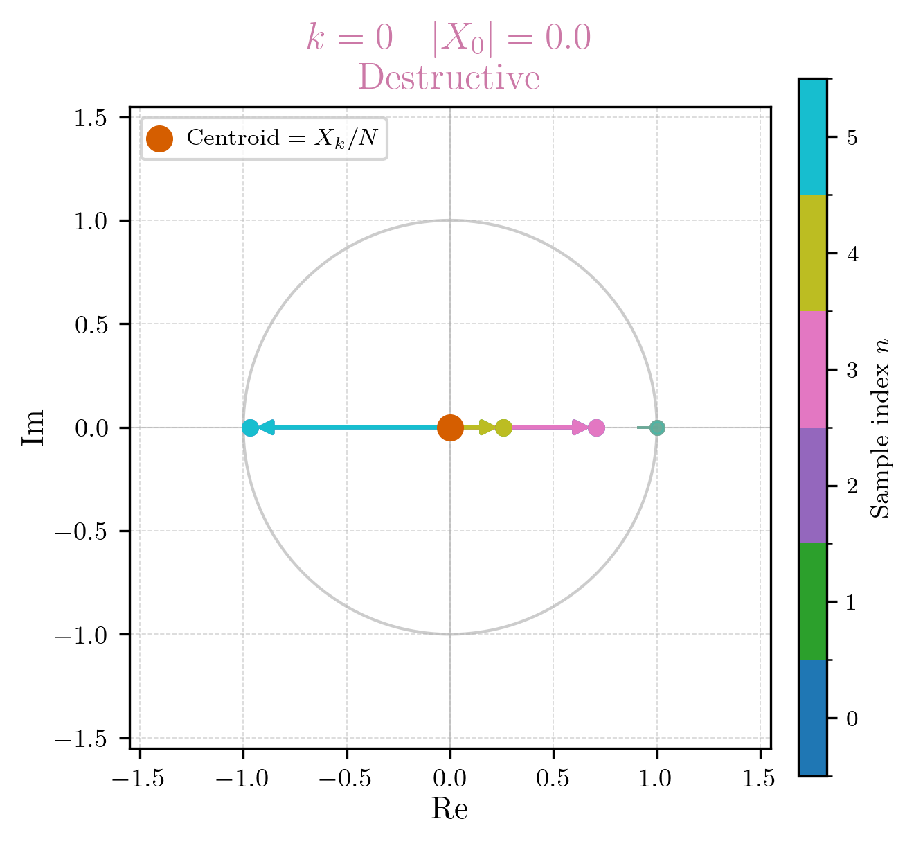
Okay so we immediately ran into a special case. For $k=0$, the complex exponential term becomes 1 for all $n$, which means that no rotation is imposed on the signal at all. Instead of capturing a specific frequency component, $X_0$ simply sums up all the samples in our signal. This is why $X_0$ is often referred to as the “DC component” of the DFT, because it captures the average value of the signal (which is 0 in our case).

It’s called DC component because in the context of electrical signals (which this entire discipline arose off of), a constant (non-varying) signal is referred to as “direct current” (DC), while a varying signal is referred to as “alternating current” (AC). The DC component of the DFT captures the constant part of the signal, while the other components capture the varying parts.

If we were to draw the summations of $X_0$ on the unit circle, it would look like this:

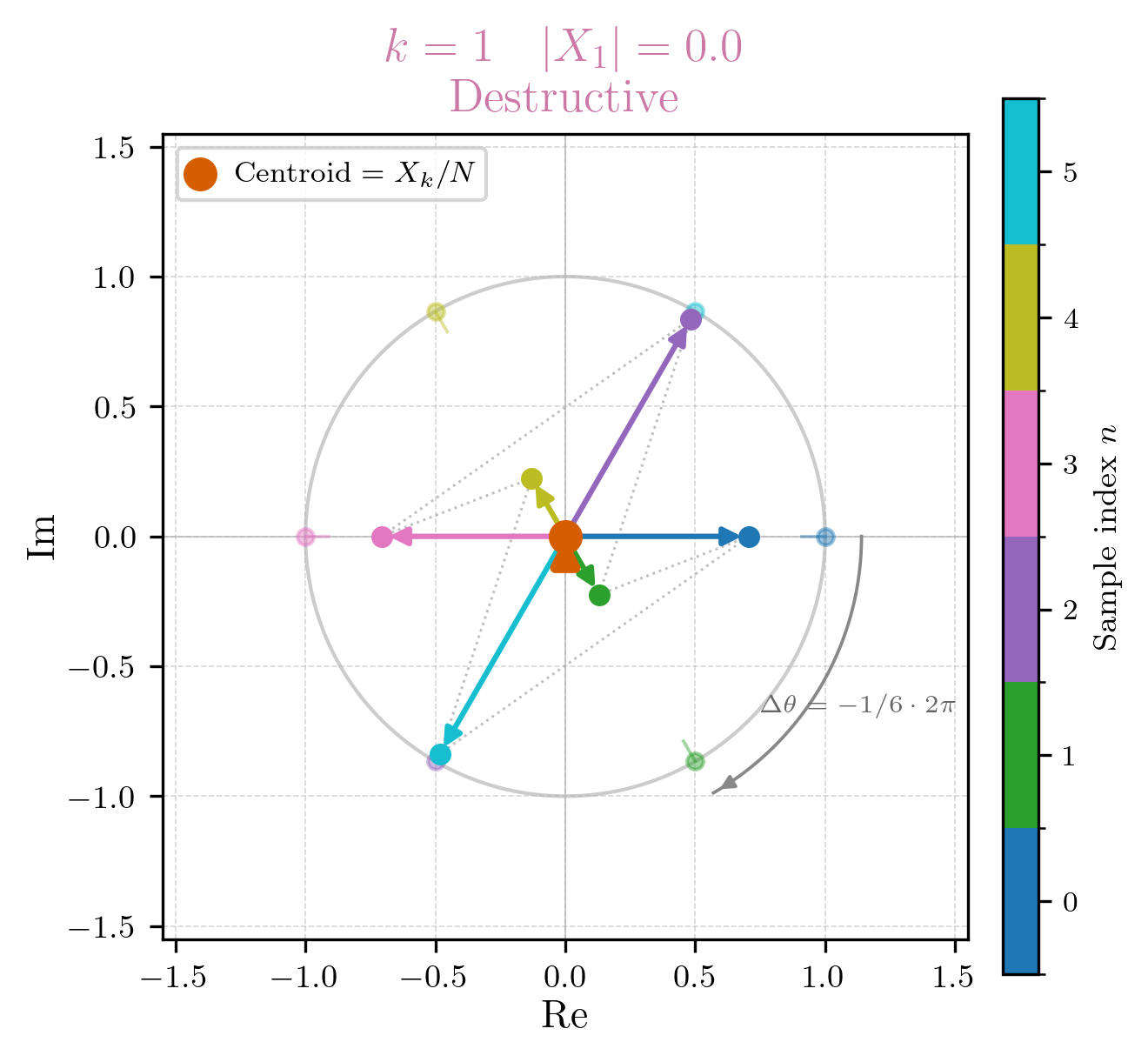
For $k=1$, it finally gets interesting. Remember, now we have a rotation of $-2\pi i\frac{n}{6}$, which means that as $n$ goes from 0 to 5, we will complete one full clockwise rotation around the unit circle. This also means that for every sample we rotate $\Delta\theta = \frac{2\pi}{6}$ radians clockwise around the unit circle. The DFT coefficient $X_1$ will capture how much of this 1 Hz frequency component is present in our signal. The calculation is as follows:

$$\begin{aligned} X_1 &= \sum_{n=0}^{5} x_n e^{-2\pi i\frac{n}{6}1} \\ &= 0.707 e^{-2\pi i\frac{0}{6}1} + 0.259 e^{-2\pi i\frac{1}{6}1} -0.966 e^{-2\pi i\frac{2}{6}1} + 0.707 e^{-2\pi i\frac{3}{6}1} + 0.259 e^{-2\pi i\frac{4}{6}1} -0.966 e^{-2\pi i\frac{5}{6}1} \\ &= 0.707 + (0.130-0.224i) + (0.483+0.836i) -0.707 + (-0.130+0.224i) + (-0.483-0.836i) \\ &= 0 \end{aligned}$$

As we can see, $X_1$ is also 0 as all the calculated values counteract eachother, which corresponds to our intuition that there is no 1 Hz component in our signal. If we were to draw the summation of $X_1$ on the unit circle, it would look like this:

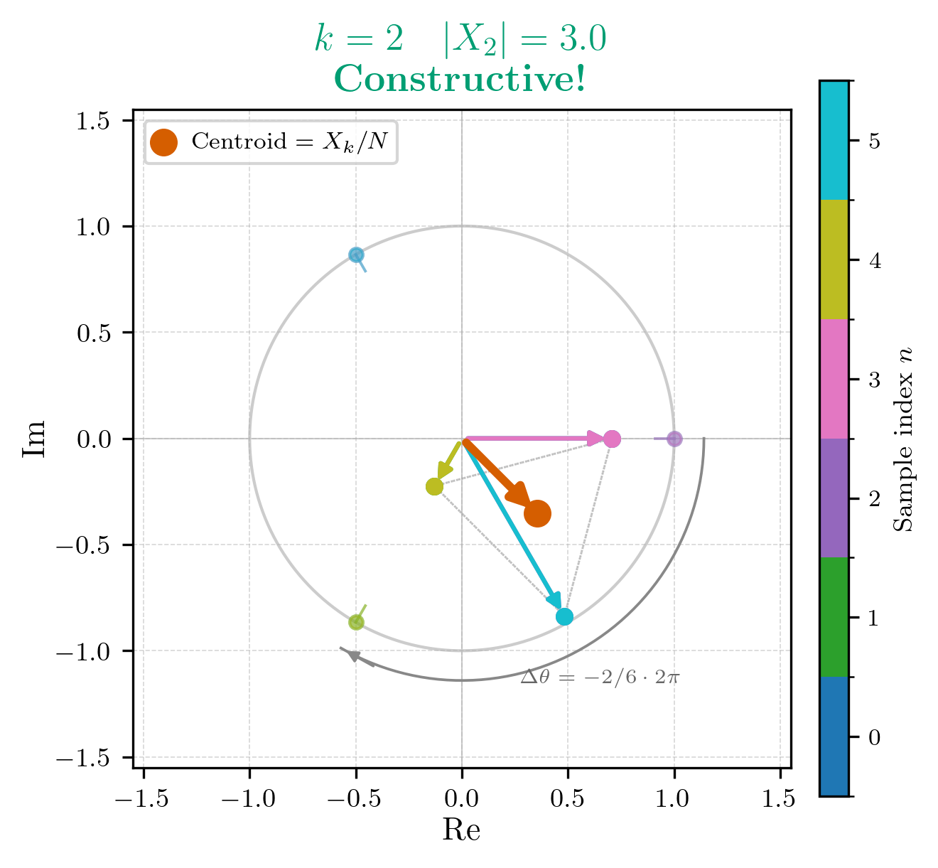
For $k=2$, we have a rotation of $-2\pi i\frac{n}{6}2$, which means that as $n$ goes from 0 to 5, we will complete two full clockwise rotations around the unit circle, with a rotation step size of $\Delta\theta = 2\frac{2\pi}{6} = \frac{2\pi}{3}$ radians. This is the frequency component that corresponds to our original 2 Hz sine wave, so we expect $X_2$ to be non-zero. The calculation is as follows:

$$\begin{aligned} X_2 &= \sum_{n=0}^{5} x_n e^{-2\pi i\frac{n}{6}2} \\ &= 0.707 e^{-2\pi i\frac{0}{6}2} + 0.259 e^{-2\pi i\frac{1}{6}2} -0.966 e^{-2\pi i\frac{2}{6}2} + 0.707 e^{-2\pi i\frac{3}{6}2} + 0.259 e^{-2\pi i\frac{4}{6}2} -0.966 e^{-2 \pi i\frac{5}{6}2} \\ &= 0.707 + (-0.130-0.224i) + (0.483-0.836i) + 0.707 + (-0.130-0.224i) + (0.483-0.836i) \\ &= 2.120 - 2.120i \end{aligned}$$

Indeed, $X_2$ is non-zero, which confirms our expectation that there is a 2 Hz component in our signal. If we were to draw the summation of $X_2$ on the unit circle, it would look like this:

For $k=3$ it should be easy to show, that $X_3=0$ as well, as there is no 3 Hz component in our signal.

Now, for $k=4$ we see something interesting. Following the same logic as before we would expect $X_4$ to be zero as well, since there is no 4 Hz component in our signal. However, if we do the calculation, we find that $X_4$ is actually equal to the complex conjugate of $X_2$:

$$\begin{aligned} X_4 &= \sum_{n=0}^{5} x_n e^{-2\pi i\frac{n}{6}4} \\ &= 0.707 e^{-2\pi i\frac{0}{6}4} + 0.259 e^{-2\pi i\frac{1}{6}4} -0.966 e^{-2\pi i\frac{2}{6}4} + 0.707 e^{-2\pi i\frac{3}{6}4} + 0.259 e^{-2\pi i\frac{4}{6}4} -0.966 e^{-2\pi i\frac{5}{6}4} \\ &= 0.707 + (-0.130+0.224i) + (0.483+0.836i) + 0.707 + (-0.130+0.224i) + (0.483+0.836i) \\ &= 2.120 + 2.120i \\ &= X_2^* \end{aligned}$$

What is going on here? Why do we have this symmetry between $X_2$ and $X_4$? The answer lies in the properties of the DFT. Specifically, the DFT has a property called “conjugate symmetry”, which states that for real-valued input signals (like our samples), the DFT coefficients satisfy the following relationship:

$$X_{N-k} = X_k^* \quad \text{for } k=1, 2, \dots, N-1.$$

Conjugate symmetry of the DFT

We start by observing that for any complex number $z=e^{i\theta}$, its complex conjugate is given by $z^*=e^{-i\theta}$. Now, as before we set

$$\theta = -2\pi i\frac{n}{N}k,$$

We can then plug in $N-k$ for $k$ in the exponent of the DFT definition:

$$\begin{aligned} \exp\!\left(-2\pi i\tfrac{n}{N}(N-k)\right) &= \exp\!\left(-2\pi i\tfrac{n}{N}N\right) \cdot \exp\!\left(2\pi i\tfrac{n}{N}k\right) \\ &= \underbrace{\exp(-2\pi i n)}_{=1 \forall n} \cdot \exp\!\left(2\pi i\tfrac{n}{N}k\right) && \text{first term is whole rotations as } n \in \mathbb{Z} \\ &= \exp\!\left(2\pi i\tfrac{n}{N}k\right) \\ &= \left[\exp\!\left(-2\pi i\tfrac{n}{N}k\right)\right]^*. \end{aligned}$$

Now, we can plug this back into the DFT definition:

$$\begin{aligned} X_{N-k} &= \sum_{n=0}^{N-1} x_n \exp\!\left(-2\pi i\tfrac{n}{N}(N-k)\right) \\ &= \sum_{n=0}^{N-1} x_n \left[\exp\!\left(-2\pi i\tfrac{n}{N}k\right)\right]^* \\ &= \left[\sum_{n=0}^{N-1} x_n \exp\!\left(-2\pi i\tfrac{n}{N}k\right)\right]^* && \text{for real inputs} \\ &= X_k^*. && \blacksquare \end{aligned}$$

For our example, since $N=6$, we have $X_{6-4} = X_2^*$, which is exactly what we observed in our calculation.

This also neatly let’s us introduce two related concepts: the Nyquist frequency and the aliasing phenomenon.

The Nyquist frequency

The Nyquist frequency gives us an upper bound on the frequencies that we can accurately capture with our sampling rate. It arises from the Nyquist–Shannon sampling theorem (which is pretty involved), and states that the highest frequency we can capture by sampling our signal is half of the sampling rate. Mathematically,

$$f_{\text{ny}} = \frac{f_s}{2}.$$

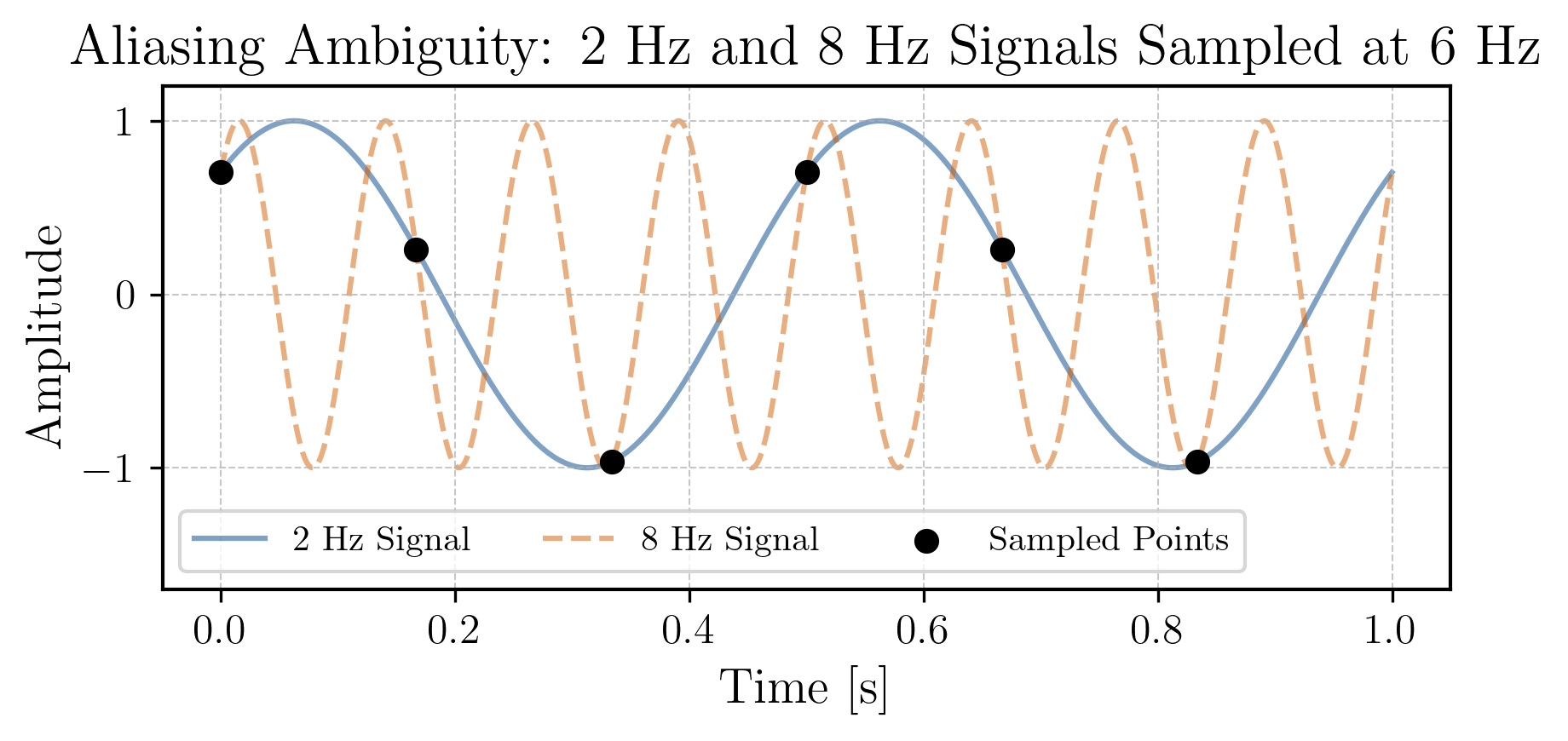
In our example, with a sampling rate of 6 Hz, the Nyquist frequency is 3 Hz. This means that we can only accurately capture frequencies up to 3 Hz with our sampling rate. If we try to capture frequencies higher than the Nyquist frequency, we will encounter the aliasing phenomenon.

You may know that the human ear is capable of hearing frequencies up to around 20 kHz, which is why audio signals are typically sampled at rates of 44.1 kHz or higher, to ensure that we can capture the full range of audible frequencies without encountering aliasing.

Aliasing phenomenon

Aliasing occurs when we try to capture frequencies higher than the Nyquist frequency. In this case, those higher frequencies will be indistinguishably mapped to lower frequencies in the DFT. In our example, if we had a 8 Hz component in our signal (that is sampled at 6 Hz), it would generate samples that are indistinguishable from a 2 Hz component, which is the same frequency as our original sine wave. You can see this in the figure below, where the 8 Hz component (in orange) is aliased to a 2 Hz component (in blue):

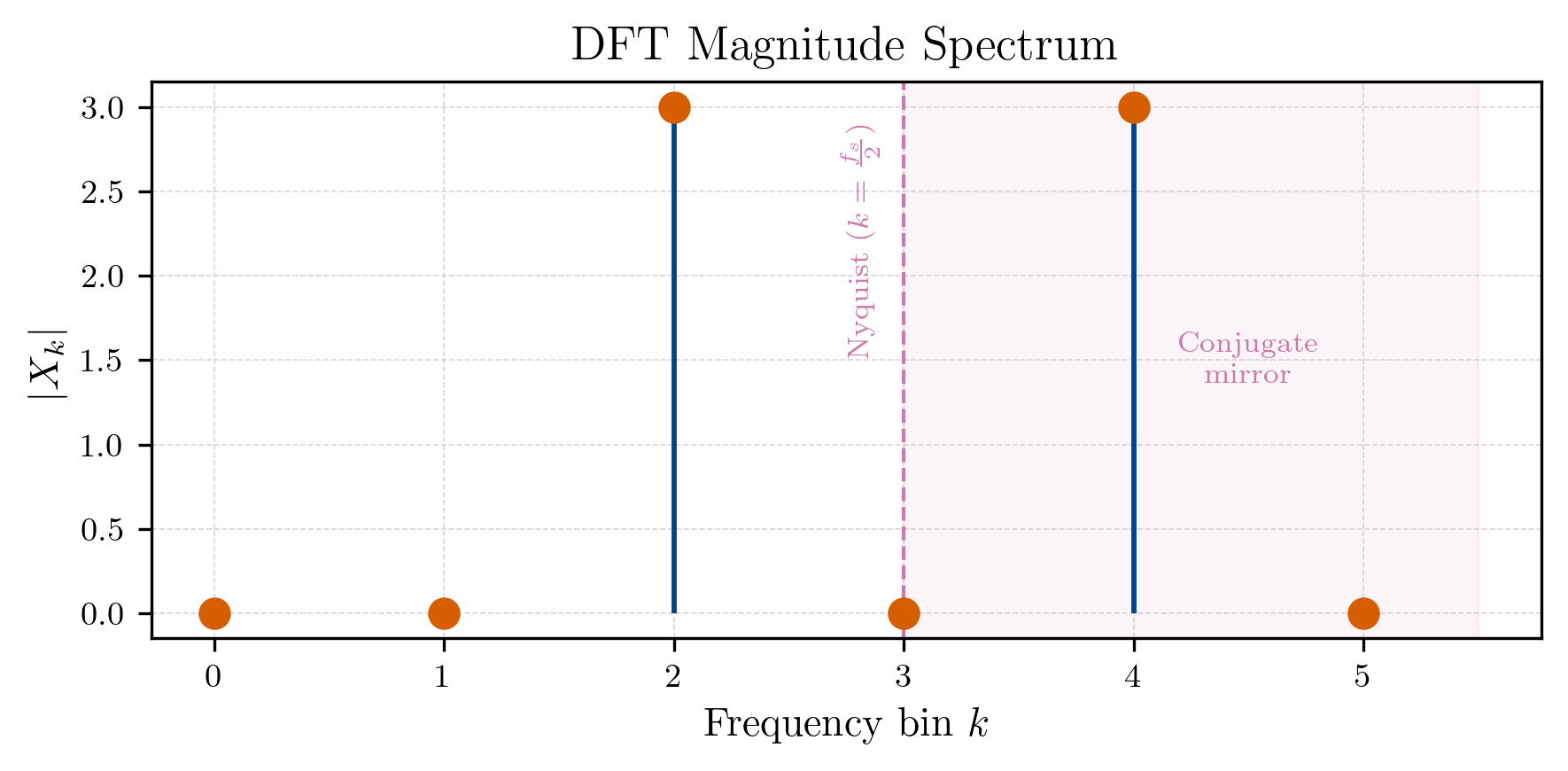
Building our spectrum

Now that we have calculated the DFT coefficients for our example signal, we can build its spectrum. The spectrum of a signal is a representation of the magnitude of its frequency components. Specifically, the magnitude of the DFT coefficient $X_k$ gives us the strength of the frequency component corresponding to $k.$ The spectrum can be visualized as a plot of the magnitudes of the DFT coefficients against their corresponding frequencies.

Recall, all the six DFT coefficients we calculated are as follows:

$$\begin{aligned} X_0 &= 0 \\ X_1 &= 0 \\ X_2 &= 2.120 - 2.120i \\ X_3 &= 0 \\ X_4 &= 2.120 + 2.120i \\ X_5 &= 0. \end{aligned}$$

The magnitude of any complex number $|a + bi|=\sqrt{a^2 + b^2}$. Therefore, the magnitudes of our DFT coefficients are:

$$\begin{aligned} |X_0| &= 0 \\ |X_1| &= 0 \\ |X_2| &= \sqrt{(2.120)^2 + (-2.120)^2} = 3 \\ |X_3| &= 0 \\ |X_4| &= \sqrt{(2.120)^2 + (2.120)^2} = 3 \\ |X_5| &= 0. \end{aligned}$$

This leaves us with the following spectrum:

Summary

In this section, we worked out why one may be interested in a mechanism like the DFT, revisited its definition, and calculated it for a simple example signal to understand how it works. We also discussed the properties of the DFT, such as conjugate symmetry, and introduced the concepts of Nyquist frequency and aliasing. In conclusion, we can say:

1. The DFT transforms a sequence of samples from the time domain to the frequency domain, allowing us to analyze the frequency components of our signal.
2. The DFT coefficients $X_k$ capture the strength of the (some cycling) frequency components corresponding to each value of $k$, which can be translated to frequencies in Hz using the sampling rate.
3. To accurately capture frequencies in our signal, we need to ensure that our sampling rate is at least twice the highest frequency present in the signal (Nyquist frequency). If we fail to do so, we will encounter the aliasing phenomenon, where higher frequencies are indistinguishably mapped to lower frequencies in the DFT.

Outlook

In the next post, I want to cover some adjacient topics of digital signal processing that we need to understand before we can start building our denoising autoencoder. Specifically, I want to talk about the Short-Time Fourier Transform (STFT), which is a variant of the DFT that allows us to analyze how the frequency content of our signal changes over time. Further I want to introduce power spectra thier visualization, and a thing called the Mel scale, all of which are important in building the input representation for our denoising autoencoder.

See you in the next one!

---

Literature

McFee, Brian. Digital Signals Theory. Chapman and Hall/CRC, 2023.