Simulating 3-DOF Ship Movements with Python 1/2

Goal and rationale

In this blog post, I want to explore how so-called Abkowitz-type maneuvering models are used for fast-time simulation of ship movements in a 2D plane, and how they are implemented in practice. The results derived here are part of my pymaneuvering suite on GitHub.

Before we start, however, I want to clarify the rationale behind this post. My goal is to foster a general understanding of the physics of simulating ship movements, the simplifications used in practice, and how these models are implemented in a programming language, in this case, Python. The section on the physical background is not required to understand the later implementation, so if you are fine with just accepting the equations governing ship movements, you can skip it and jump directly to the implementation section.

Disclaimer: Most of the physical derivations are a shameless reconstruction of the ones found in the “Bible” of marine hydrodynamics “Handbook of marine craft hydrodynamics and motion control.” written by Thor I. Fossen in 2011.

Physical background

If you ever took a basic physics class, you probably remember Newton’s golden rule: Force equals mass times acceleration

$$F=ma.$$

As a basic example (which we will go back to very soon) you can imagine pushing a block of wood across your table. If you want to move it, you push it. If the block is heavier, you push harder. In this example, pushing the block will make it just move forward. A ship at sea, however, can move in six directions simultaneously; it translates in three directions (surge, sway, heave), and rotates around three axes (yaw, roll, pitch). See Fig. 1 below for a visualization.

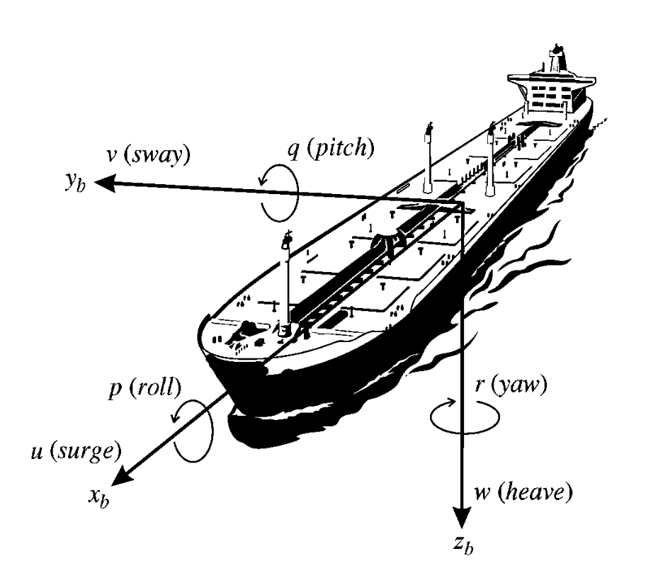
For this post, as the reader already found in the title, we will focus on implementing a 3-DOF (degree of freedom) model that only maps motions to the two-dimensional plane. The respective degrees of freedom we care about are surge, sway, and yaw. For many applications, such as path-following, path-planning, or trajectory generation, this simplification of the world is justified, as these models are generally tested in calm waters, where the third-dimension variables like heave roll and pitch are less pronouced due to missing waves.

With this simplification out of the way, we can start to actually derive the equations of motion for our case. Starting from Newton’s second law above, it is naturally defined at the Center of Gravity (CG) with respect to an inertial reference frame $i$. With a slight change of notation, we write:

$$\boldsymbol{F} = m\frac{{}^i d\boldsymbol{v}_g}{dt}$$

where $\boldsymbol{v}_g$ is the velocity of the ship at the CG. However, for practical reasons, we want to express the equations of motion in a body-fixed reference frame $b$ that is attached to the ship. This is also where we define the state variables of our system. The velocity of the origin $v$ and the rotation rate $\omega$ in the body-fixed frame are:

$$\boldsymbol{v} = \begin{bmatrix} u \\ v \\ 0 \end{bmatrix}, \qquad \boldsymbol{\omega} = \begin{bmatrix} 0 \\ 0 \\ r \end{bmatrix}.$$

The position of of the CG with respect to the body-fixed frame is given by $\boldsymbol{r}_g = [x_g, y_g, 0]^\top$. Note: The last entry of the velocity and CG position vectors as well as the the first two entries of the rotation rate vector are zero because we are only interested in the 3-DOF model, which only considers surge, sway, and yaw. The other degrees of freedom (heave, roll, pitch) are neglected. For $\boldsymbol{r}_g$ this means that our CG is some point on the plane.

The velocity of the CG is related to the velocity of the origin and the rotation rate by the following equation:

$$\begin{aligned} \boldsymbol{v}_g &= \boldsymbol{v} + \boldsymbol{\omega} \times \boldsymbol{r}_g \\ &= \begin{bmatrix} u- y_g r \\ v + x_g r \\ 0 \end{bmatrix} \end{aligned}$$

Derivation: calculating the velocity of the CG in the inertial frame

$$\begin{aligned} \boldsymbol{v}_g &= \boldsymbol{v} + \boldsymbol{\omega} \times \boldsymbol{r}_g \\ &= \begin{bmatrix} u \\ v \\ 0 \end{bmatrix} + \begin{bmatrix} 0 \\ 0 \\ r \end{bmatrix} \times \begin{bmatrix} x_g \\ y_g \\ 0 \end{bmatrix} \\ &= \begin{bmatrix} u \\ v \\ 0 \end{bmatrix} + \begin{bmatrix} -r y_g \\ r x_g \\ 0 \end{bmatrix} \\ &= \begin{bmatrix} u - y_g r \\ v + x_g r \\ 0 \end{bmatrix} \end{aligned}$$

To now express newton’s second law in the body-fixed frame, we need to apply the transport theorem, which states that the time derivative of a vector in an inertial frame can be expressed as the time derivative of the same vector in a rotating frame plus the cross product of the rotation rate and the vector itself. Applying this to our case, we get:

$$\begin{aligned} \frac{{}^i d\boldsymbol{v}_g}{dt} &= \frac{{}^b d\boldsymbol{v}_g}{dt} + \boldsymbol{\omega} \times \boldsymbol{v}_g \\ &= \begin{bmatrix} \dot{u} - y_g \dot{r} - r v - x_g r^2 \\ \dot{v} + x_g \dot{r} + r u - y_g r^2 \\ 0 \end{bmatrix} \end{aligned}$$

Derivation: applying the transport theorem

$$\begin{aligned} \frac{{}^i d\boldsymbol{v}_g}{dt} &= \frac{{}^b d\boldsymbol{v}_g}{dt} + \boldsymbol{\omega} \times \boldsymbol{v}_g \\ &= \begin{bmatrix} \dot{u} - y_g \dot{r} \\ \dot{v} + x_g \dot{r} \\ 0 \end{bmatrix} + \begin{bmatrix} 0 \\ 0 \\ r \end{bmatrix} \times \begin{bmatrix} u - y_g r \\ v + x_g r \\ 0 \end{bmatrix} \\ &= \begin{bmatrix} \dot{u} - y_g \dot{r} \\ \dot{v} + x_g \dot{r} \\ 0 \end{bmatrix} + \begin{bmatrix} -r (v + x_g r) \\ r (u - y_g r) \\ 0 \end{bmatrix} \\ &= \begin{bmatrix} \dot{u} - y_g \dot{r} - r v - x_g r^2 \\ \dot{v} + x_g \dot{r} + r u - y_g r^2 \\ 0 \end{bmatrix} \end{aligned}$$

Now all thats left is to multiply the mass $m$ with the acceleration to get the forces in the body-fixed frame:

$$\begin{aligned} \boldsymbol{F} &= m\frac{{}^i d\boldsymbol{v}_g}{dt} \\ &= m \begin{bmatrix} \dot{u} - y_g \dot{r} - r v - x_g r^2 \\ \dot{v} + x_g \dot{r} + r u - y_g r^2 \\ 0 \end{bmatrix} \end{aligned}$$

In the literature, the longitudinal and lateral forces are usually denoted by $X$ and $Y$. If we follow this convention, we can write the equations of motion as:

$$\begin{aligned} X &= m (\dot{u} - y_g \dot{r} - r v - x_g r^2) \\ Y &= m (\dot{v} + x_g \dot{r} + r u - y_g r^2) \end{aligned} \tag{1}$$

The derivation for the moments is a bit more involved, but it follows the same principles as above. You can find the detailed derivation in Fossen’s book in Chapter 3. The final equations of motion for the moments are:

$$\begin{aligned}N &= I_z \dot{r} + m [x_g (\dot{v} + ur) - y_g (\dot{u} - vr)] \end{aligned}\tag{2}$$

where $I_z$ is the moment of inertia around the z-axis.

What about the forces and moments?

The equations above only describe the kinematics of the ship, i.e., how the ship moves given the forces and moments acting on it. To actually simulate the ship’s movement, we must somehow estimate the forces and moments acting on the ship. For this to work, we need two ingedients:

1. A maneuvering model that maps the state of the ship to the forces and moments acting on it. For fast-time simulations, these are usually black- or grey box coefficient models like the Abkowitz-type (aha, we’re getting closer) and MMG models.

2. An estimation model that can produce the coefficients we need to put into the maneuvering model.

Note: In this blog, we leave out the estimation model, as it is a topic of its own. For now, we just note, that the model we introduce in the next section was calibrated using a captive model test and computational fluid dynamics (CFD) simulations.

The Abkowitz-type maneuvering model

For our first ingedient, the maneuvering model, we will use an Abkowitz-type model. The original model was developed by Abkowitz (1964) and is based on empirical data from towing tank experiments. It is a black-box model that maps the state of the ship to the forces and moments acting on it using a taylor expansion around an equilibrium speed. They are called black-box models because they do not explicitly model the physics of the forces and moments, but rather model them as a function of the state variables. The coefficients of the taylor expansion are usually estimated using regression techniques on experimental data. The specific equations we use today are taken from Yang (2023) as they prepare us the shallow-water correction of Yang (2024) which we will cover in a different post. The equations are as follows:

$$\begin{aligned} X &= X_0 + X_{\dot{u}}\dot{u} + X_u \Delta u + X_{uu} \Delta u^2 + X_{vv} v^2 + X_{vvvv} v^4 + X_{rr} r^2 + X_{vr} vr \\ &\quad + X_{vvrr} v^2 r^2 + X_{\delta\delta} \delta^2 + X_{u\delta\delta} \Delta u \delta^2 \\ Y &= Y_0 + Y_{\dot{v}}\dot{v} + Y_{\dot{r}}\dot{r} + Y_v v + Y_{vvv} v^3 + Y_r r + Y_{rrr} r^3 \\ &\quad + Y_{vrr} vr^2 + Y_{vvr} v^2 r + Y_{\delta} \delta + Y_{\delta\delta\delta} \delta^3 + Y_{u\delta} \Delta u \delta + Y_{u\delta\delta\delta} \Delta u \delta^3 \\ N &= N_0 + N_{\dot{v}}\dot{v} + N_{\dot{r}}\dot{r} + N_v v + N_{vvv} v^3 + N_r r + N_{rrr} r^3 \\ &\quad + N_{vrr} vr^2 + N_{vvr} v^2 r + N_{\delta} \delta + N_{\delta\delta\delta} \delta^3 + N_{u\delta} \Delta u \delta + N_{u\delta\delta\delta} \Delta u \delta^3 \end{aligned}\tag{3}$$

Okay, I know that’s a lot of coefficients, but trust me in saying that we already know almost everything in this model. All the variables with subscripts ($X_{vvr}, Y_{u\delta\delta\delta}$, etc.) are called “hydrodynamic derivatives” and they are provided to us by the authors of the paper who have measured them in their experiments (also, conveniently, $X_0=Y_0 =N_0=0$). The only remaining variables are $\delta$ which is just the rudder angle, and $\Delta u$ which is the difference between the current surge velocity and the equilibrium surge velocity used for the taylor expansion (i.e., $\Delta u = u - U_0$; in our example the authors measured the model at $U_0=2.777 m/s$).

Detour: Non-dimensionalization

I must briefly talk about non-dimensionalization. It is a standard procedure in ship maneuvering modeling used to generalize the equations of motion by scaling dimensional variables, such as surge velocity ($u$), hydrodynamic forces ($X,Y$), and moments ($N$), against characteristic reference values including fluid density ($\rho$), the ship’s length between perpendiculars (L), and the equilibrium surge velocity ($U_0$​). By introducing dimensionless variables, the mathematical framework becomes independent of specific units and physical scale, facilitating direct performance comparisons across diverse hull forms and operating conditions. This process ensures numerical consistency when evaluating hydrodynamic derivatives within a Taylor series expansion, providing a more robust foundation for simulation and stability analysis.

Our framework for non-dimensionalization is as follows:

$$u' = \frac{u}{U}, \quad v' = \frac{v}{U}, \quad r' = \frac{rL}{U} \quad \Delta u' = \frac{\Delta u}{U} \quad \text{and} \quad F' = \frac{F}{0.5\rho U^2 L^2}, \quad M' = \frac{M}{0.5\rho U^2 L^3}$$

where $U=\sqrt{u^2+v^2}$, $\rho$ is the fluid density, and $L$ is the ship’s length between perpendiculars. The non-dimensionalized equations of motion can then be expressed in terms of these dimensionless variables, allowing for a more generalized analysis of ship maneuvering behavior.

What this means for us in practice is that we need to non-dimensionalize the state variables from the Abkowitz model equations for the forces and moments before actually calculating them. Only once all the force and moment terms are calculated, we can re-dimensionalize them to get the actual forces and moments acting on the ship.

Solving the equations of motion

Now, you might be asking yourself, how do we combine all the information we have so far to actually simulate the ship’s movement? Since we now have all ingredients in place we can make a plan:

The goal will be to transform equations (1), (2) and (3) into a linear system of the form

$$\boldsymbol{M} \boldsymbol{\dot{\nu}} = \boldsymbol{F}$$

where $\boldsymbol{M}$ is the mass matrix, $\boldsymbol{\dot{\nu}}=[\dot{u}, \dot{v}, \dot{r}]^\top$ is the vector of accelerations, and $\boldsymbol{F} = [X,Y,N]^\top$ is the vector of forces and moments. Once we have this linear system, we can solve for the accelerations $\boldsymbol{\dot{\nu}}$ by multiplying both sides of the equation by the inverse of the mass matrix $\boldsymbol{M}^{-1}$:

$$\boldsymbol{\dot{\nu}} = \boldsymbol{M}^{-1} \boldsymbol{F}.$$

You may have aleady noticed that our forces and moments $X$, $Y$, and $N$ are not just functions of the state variables, but also of their derivatives (i.e., $\dot{u}$, $\dot{v}$, $\dot{r}$). So in a first step, we need to rearrange the equations to get all the derivative terms on the left-hand side and all the non-derivative terms on the right-hand side. From now on, I will always look at equations (1) and (2) together, as they are closely related.

$$\begin{aligned} m (\dot{u} - y_g \dot{r} - r v - x_g r^2) &= X \\ m (\dot{v} + x_g \dot{r} + r u - y_g r^2) &= Y \\ I_z \dot{r} + m [x_g (\dot{v} + ur) - y_g (\dot{u} - vr)] &= N \end{aligned}$$

Looking at (3) we will now pull out all the derivative terms, while hiding the non-derivative terms in a new variable $F_{rest}$:

$$\begin{aligned} m (\dot{u} - y_g \dot{r} - r v - x_g r^2) &= X_{\dot{u}}\dot{u} + X_{rest} \\ m (\dot{v} + x_g \dot{r} + r u - y_g r^2) &= Y_{\dot{v}}\dot{v} +Y_{\dot{r}}\dot{r} + Y_{rest} \\ I_z \dot{r} + m [x_g (\dot{v} + ur) - y_g (\dot{u} - vr)] &= N_{\dot{v}}\dot{v} + N_{\dot{r}}\dot{r} + N_{rest} \end{aligned}$$

Now, remember that in order to solve our linear equation, we only need terms related to the derivatives on the left-hand side. Everything else can be moved to the right-hand side. So we can rearrange the equations and group by derivatives to get:

$$\begin{aligned} (m - X_{\dot{u}})\dot{u} + (-m y_g)\dot{r} &= X_{rest} + mrv + m x_g r^2 \\ (m - Y_{\dot{v}})\dot{v} + (m x_g - Y_{\dot{r}})\dot{r} &= Y_{rest} - mru + m y_g r^2 \\ (I_z - N_{\dot{r}})\dot{r} + (m x_g - N_{\dot{v}})\dot{v} + (-m y_g) \dot{u} &= N_{rest} - m x_g ur + m y_g vr \end{aligned}\tag{4}$$

Derivation: rearranging the equations of motion

$$\left. \begin{aligned} m (\dot{u} - y_g \dot{r} - r v - x_g r^2) &= X_{\dot{u}}\dot{u} + X_{rest} \\ m (\dot{v} + x_g \dot{r} + r u - y_g r^2) &= Y_{\dot{v}}\dot{v} +Y_{\dot{r}}\dot{r} + Y_{rest} \\ I_z \dot{r} + m [x_g (\dot{v} + ur) - y_g (\dot{u} - vr)] &= N_{\dot{v}}\dot{v} + N_{\dot{r}}\dot{r} + N_{rest} \end{aligned}\right\}$$

Expand the left-hand side:

$$\left. \begin{aligned} m\dot{u} - m y_g \dot{r} - mrv - m x_g r^2 &= X_{\dot{u}}\dot{u} + X_{rest} \\ m \dot{v} + m x_g \dot{r} + m r u - m y_g r^2 &= Y_{\dot{v}}\dot{v} +Y_{\dot{r}}\dot{r} + Y_{rest} \\ I_z \dot{r} + m x_g \dot{v} + m x_g ur - m y_g \dot{u} - m y_g vr &= N_{\dot{v}}\dot{v} + N_{\dot{r}}\dot{r} + N_{rest} \end{aligned}\right\}$$

Move all terms from the left-hand-side not containing a derivative to the right-hand-side and all terms from the right-hand-side containing a derivative to the left-hand-side:

$$\left. \begin{aligned} m\dot{u} - m y_g \dot{r} - X_{\dot{u}}\dot{u} &= X_{rest} + mrv + m x_g r^2 \\ m \dot{v} + m x_g \dot{r} - Y_{\dot{v}}\dot{v} - Y_{\dot{r}}\dot{r} &= Y_{rest} - mru + m y_g r^2 \\ I_z \dot{r} + m x_g \dot{v} - m y_g \dot{u} - N_{\dot{v}}\dot{v} - N_{\dot{r}}\dot{r} &= N_{rest} - m x_g ur + m y_g vr \end{aligned}\right\}$$

With all terms on the correct sides of the equations, the only thing left is to group by derivative to find the coefficients of $\boldsymbol{M}$:

$$\left. \begin{aligned} (m - X_{\dot{u}})\dot{u} + (-m y_g)\dot{r} &= X_{rest} + mrv + m x_g r^2 \\ (m - Y_{\dot{v}})\dot{v} + (m x_g - Y_{\dot{r}})\dot{r} &= Y_{rest} - mru + m y_g r^2 \\ (I_z - N_{\dot{r}})\dot{r} + (m x_g - N_{\dot{v}})\dot{v} + (-m y_g) \dot{u} &= N_{rest} - m x_g ur + m y_g vr \end{aligned}\right\}$$

From (4) it should now be straight forward to construct our mass matrix

$$\boldsymbol{M}= \begin{bmatrix} m-X_{\dot{u}} & 0 & -m y_g \\ 0 & m - Y_{\dot{v}} & m x_g - Y_{\dot{r}} \\ -m y_g & m x_g - N_{\dot{v}} & I_z - N_{\dot{r}} \end{bmatrix},\tag{5}$$

and our force vector

$$\boldsymbol{F} = \begin{bmatrix} X_{rest} + mrv + m x_g r^2 \\ Y_{rest} - mru + m y_g r^2 \\ N_{rest} - m x_g ur + m y_g vr \end{bmatrix}.\tag{6}$$

Now we are all set to implement the model in Python.

Implementation

With the physics out of the way, we can move on to the implementation. As mentioned in the introduction, the goal here is to understand how the code in my pymaneuvering library works and what it is based on. For this post, however, we will at first only look at the implementation of the Abkowitz-type model for deep water. The shallow-water correction (which is actually implemented in the library) will be covered in a different post.

So, the first thing we need is some object resembling our ship, holding all the necessary parameters and coefficients . For the inland barge modeled in Yang (2024) we look at Tables 1 and 2 for reference. In my implementation, I use a dataclass:

from dataclasses import dataclass
@dataclass
class ShipParameters:
    # Reference Speed and Properties
    U_0: float = 2.777 # Reference speed
    L: float = 105.0 # Length
    B: float = 9.5 # Width
    T: float = 2.8 # Draft
    x_G: float = 0.887 # Longitudinal center of gravity [m]
    m: float = 2478451.0
    r_zz: float = 24.526 # Radius of gyration around z [m]
    rho: float = 1000.0

    # --- Surge Force (X) Coefficients ---
    X_0: float = 0.0
    X_udot: float = -12.3e-5
    X_u: float = -220.1e-5
    X_uu: float = 72.4e-5
    X_vv: float = -73.3e-5
    X_vvvv: float = 0.0
    X_rr: float = -4.7e-5
    X_vr: float = 279.2e-5
    X_vvrr: float = 44.5e-5
    X_dd: float = -88.7e-5
    X_udd: float = 290.0e-5

    # --- Sway Force (Y) Coefficients ---
    Y_0: float = 0.0
    Y_vdot: float = -311.7e-5
    Y_rdot: float = -4.2e-5
    Y_v: float = -782.3e-5
    Y_vvv: float = -2814.1e-5
    Y_r: float = 60.6e-5
    Y_rrr: float = 23.4e-5
    Y_vrr: float = -410.8e-5
    Y_vvr: float = 1058.2e-5
    Y_d: float = 135.7e-5
    Y_ddd: float = -56.6e-5
    Y_ud: float = -289.5e-5
    Y_uddd: float = 98.5e-5

    # --- Yaw Moment (N) Coefficients ---
    N_0: float = 0.0
    N_vdot: float = -4.2e-5
    N_rdot: float = -19.3e-5
    N_v: float = -230.8e-5
    N_vvv: float = 0.0
    N_r: float = -90.9e-5
    N_rrr: float = -40.4e-5
    N_vrr: float = -101.1e-5
    N_vvr: float = -833.2e-5
    N_d: float = -64.4e-5
    N_ddd: float = 27.1e-5
    N_ud: float = 139.8e-5
    N_uddd: float = -47.5e-5

One thing the eagle-eyed may have already noticed is that we are missing the lateral distance to the center of gravity $y_g$ in our dictionary. Many papers on ship maneuvering modeling assume that the CG is located on the centerline of the ship, which means that $y_g=0$. This is also the case in our example. You will later see that this simplifies our equations of motion quite a bit. Let us quickly import the necessary libraries:

import numpy as np
import math
from numpy.typing import NDArray

But now we need to define the actual function that evolves the state of the ship. According to (4), we need the following inputs to our function for this to work. Our current surge and sway velocities, as well as our yaw rate packed in one vector $\boldsymbol{\nu} = [u,v,r]^\top$, the rudder angle $\delta$ in radians (of course we need this, because otherwise we wouldn’t be able to actually control the ship), and information about the ship itself. The signature will be

def dynamics(vessel: ShipParameters, 
             nu: NDArray[np.float32], 
             delta: float) -> NDArray[np.float32]:

Before we calculate the forces and moments, we need to define some variables which we will need for the non-dimensionalized calculation

u, v, r  = nu

# Shorten the parameter dict to avoid clutter later
p = vessel
        
# Difference from reference speed
du = u - p.U_0

# Instantaneous speed
U = math.sqrt(u**2 + v**2) + 1e-6 # Add small number to avoid division by zero at U=0
        
# Non-dimensionalized quantities
v_prime = v / U
r_prime = r * p.L / U
du_prime = du / U

Now we can just copy $X_{rest},Y_{rest}$ and $N_{rest}$ from (4) to the code

# Force in the X-direction (Longitudinal)
F_X = (p.X_u * du_prime + p.X_uu * du_prime**2 + 
       p.X_vv * v_prime**2 + p.X_vvvv * v_prime**4 + p.X_rr * r_prime**2 + 
       p.X_vr * v_prime * r_prime + p.X_vvrr * v_prime**2 * r_prime**2 + 
       p.X_dd * delta**2 + p.X_udd * du_prime * delta**2)

# Force in the Y-direction (Lateral)
F_Y = (p.Y_v * v_prime + 
       p.Y_vvv * v_prime**3 + p.Y_r * r_prime + p.Y_rrr * r_prime**3 + 
       p.Y_vrr * v_prime * r_prime**2 + p.Y_vvr * v_prime**2 * r_prime + 
       p.Y_d * delta + p.Y_ddd * delta**3 + 
       p.Y_ud * du_prime * delta + p.Y_uddd * du_prime * delta**3)

# Yaw Moment (N)
F_N = (p.N_v * v_prime + 
       p.N_vvv * v_prime**3 + p.N_r * r_prime + p.N_rrr * r_prime**3 + 
       p.N_vrr * v_prime * r_prime**2 + p.N_vvr * v_prime**2 * r_prime + 
       p.N_d * delta + p.N_ddd * delta**3 + 
       p.N_ud * du_prime * delta + p.N_uddd * du_prime * delta**3)

Belive it or not, we are almost done already. We just need to perform one final stretch to re-dimensionalize the forces and calculate the moment of intertia for our ship. The moment of inertia will be calculated via the ship’s radius of gyration $r_{zz}$. The well known formula for the moment of inertia is $I_z = m r_{zz}^2$.

# Moment of inertia in yaw from radius of gyration
I_zz = p.m * p.r_zz**2

For the re-dimensionalization, we need to multiply the non-dimensionalized forces and moments with the respective reference values provided in the non-dimensionalization section above:

# Dimensionalizers
D_FORCE  = 0.5 * p.rho * U**2 * p.L**2
D_MOMENT = 0.5 * p.rho * U**2 * p.L**3

# Re-dimensionalize forces and moments
F_X = F_X * D_FORCE
F_Y = F_Y * D_FORCE
F_N = F_N * D_MOMENT

Detour: Re-dimensionalization of the added mass coefficients

The right-hand side of our linear system is now complete, we just need to construct the mass matrix $\boldsymbol{M}$. Inside this matrix we find coefficients like $X_{\dot{u}}$, $Y_{\dot{v}}$, etc., which are called “added mass coefficients”. They are called this way because they can be interpreted as the additional mass that the ship needs to accelerate due to the fact that it is moving through a fluid. The added mass coefficients are usually negative, which means, due to double negativity, that they increase the effective mass of the ship, because it needs to accelerate not only itself, but also some of the surrounding fluid. The rest are called “cross-terms” and represent the coupling between different degrees of freedom. For example, $Y_{\dot{r}}$ represents the coupling between the yaw rate and the sway force, which means that if the ship is rotating, it will also experience a lateral force.

To re-dimensionalize them, we must understand what units they are in. Added masses like $X_{\dot{u}}$, or $Y_{\dot{v}}$ add to the intertia of the ship. If we want to accelerate the ship in surge, we need to accelerate not only the mass of the ship, but also parts of the water around it. According to the laws of fluid mechanics, the force required to accelerate the fluid is directly proportional to the acceleration of the body. See this example for surge velocity:

$$F_{fluid} = X_{\dot{u}} \dot{u}$$

To see what units $X_{\dot{u}}$ must be in, we can rearrange the equation to solve for $X_{\dot{u}}$:

$$X_{\dot{u}} = \frac{F_{fluid}}{\dot{u}} \stackrel{units}{=} \frac{[ML/T^2]}{[L/T^2]} = [M] = kg,$$

where $[M]$ represents the unit of mass, $[L]$ represents the unit of length, and $[T]$ represents the unit of time.

As with the non-dimensionalization, we need to reconstruct our variables using the “building blocks” of our system’s environment, water density $\rho$, the ship’s length $L$, and the reference speed $U$.

Sticking to our example of $X_{\dot{u}}$, we must somehow get from a dimensionless coefficient to a coefficient with units of mass, just by combining the building blocks. One way is to use $\rho$ which is of units $[M/L^3]$, and $L$ which is of units $[L]$:

$$[M/L^3] \times [L]^3 = [M]$$

This way we build the re-dimensionalization factor for the added mass coefficients as $\rho L^3$. The same logic can be applied to the other terms to arrive at the following re-dimensionalization factors:

Coefficient Type	Re-dimensionalization Factor
Added Mass Coefficients ($X_{\dot{u}}$, $Y_{\dot{v}}$)	$0.5\rho L^3$
Cross-Terms ($Y_{\dot{r}}$, $N_{\dot{v}}$)	$0.5\rho L^4$
Intertia Terms ($N_{\dot{r}}$)	$0.5\rho L^5$

The 0.5 is a convention carried over from the kinetic energy definition $\frac{1}{2}mv^2$ and dynamic pressure $q = \frac{1}{2} \rho U^2$.

Back to the implementation

With the knowledge of the re-dimensionalization factors, we can now apply them and build the mass matrix $\boldsymbol{M}$:

# Re-dimensionalize added mass couplings
am_surge  = p.X_udot * 0.5 * p.rho * (p.L**3)
am_sway_v = p.Y_vdot * 0.5 * p.rho * (p.L**3)
am_sway_r = p.Y_rdot * 0.5 * p.rho * (p.L**4)
am_yaw_v  = p.N_vdot * 0.5 * p.rho * (p.L**4)  
am_yaw_r  = p.N_rdot * 0.5 * p.rho * (p.L**5)

# Eq (5) with re-dimensionalized added mass coefficients
M = np.array(
    [
        [p.m - am_surge, 0.0,                    0.0                    ],
        [0.0,            p.m - am_sway_v,        p.m * p.x_G - am_sway_r],
        [0.0,            p.m * p.x_G - am_yaw_v, I_zz - am_yaw_r        ]
    ]
)

As I promised, you see that the bottom left and the top right entries of the mass matrix are zero, because we have assumed that $y_g=0$.

Our force vector $\boldsymbol{F}$ had some simplifications as well, because of the same assumption. If we look at (6) we see that all terms containing $y_g$ are zero, which simplifies our force vector to:

# Eq (6) without terms containing y_g
F = np.array(
    [
        F_X + p.m * v * r + p.m * p.x_G * (r**2),
        F_Y - p.m * u * r,
        F_N - p.m * p.x_G * u * r
    ]
)

The only thing left is to solve the system and return the accelerations:

# Solve for accelerations
return np.linalg.solve(M, F)

Simulation

With the dynamics function defined, we can now simulate the ship’s movement over time. The only thing we need to carefully do is to transform the body-fixed accelerations we get from the dynamics function to the inertial frame, which is the frame we want to visualize our ship’s movement in. As per Fossen (2011), the transformation from body-fixed velocities to inertial velocities for a given heading $\psi$ is given by:

$$R(\psi) = \begin{bmatrix} \cos\psi & -\sin\psi & 0 \\ \sin\psi & \cos\psi & 0 \\ 0 & 0 & 1 \end{bmatrix}$$

Therefore, for a given position and heading of the ship $\boldsymbol{\eta} = [x, y, \psi]^T$, the transformation from body-fixed velocities $\boldsymbol{\nu} = [u, v, r]^T$ to inertial velocities $\dot{\boldsymbol{\eta}}$ is given by:

$$\dot{\boldsymbol{\eta}} = R(\psi) \boldsymbol{\nu}$$

In code:

def rotpsi(psi: float) -> NDArray[np.float32]:
    return np.array(
        [
            [np.cos(psi), -np.sin(psi), 0.0],
            [np.sin(psi),  np.cos(psi), 0.0],
            [0.0,          0.0,         1.0]
        ]
    )

For the simulation, we will employ a standard velocity verlet integration scheme and simulate 500 timesteps with a timestep of 1.0 second:

def velocity_verlet_integration(
    vessel: ShipParameters, 
    nu: NDArray[np.float32], 
    delta: float,
    pos: NDArray[np.float32],
    psi: float,
    dT: float) -> tuple[NDArray[np.float32], NDArray[np.float32]]:
        """
        Implements Velocity Verlet for surge, sway, yaw (Nu) and X, Y, Heading (Eta).
        """
        # nu = [u, v, r]
        # pos = [X, Y]
        # psi = heading [rad]
        
        # Current acceleration (Nu_dot) at time t
        nu_dot_t = dynamics(vessel=vessel, nu=nu, delta=delta)
        
        # Rotation matrix at current heading
        R_t = rotpsi(psi)
        
        # Global velocity (Eta_dot) and Global acceleration (Eta_ddot) at time t
        eta_dot_t = np.dot(R_t, nu)
        eta_ddot_t = np.dot(R_t, nu_dot_t)

        # 2. UPDATE POSITION (eta)
        # Eta(t + dt) = Eta(t) + Eta_dot(t)*dt + 0.5 * Eta_ddot(t) * dt^2
        eta_current = np.append(pos, psi)
        new_eta = eta_current + eta_dot_t * dT + 0.5 * eta_ddot_t * (dT**2)
        
        # Normalize heading
        new_eta[2] = angle_to_two_pi(new_eta[2]) # This is for the reader :) 

        # 3. Half-step velocity (nu)
        # Nu_mid = Nu(t) + 0.5 * Nu_dot(t) * dt
        nu_mid = nu + 0.5 * nu_dot_t * dT

        # 4. New Acceleration 
        # Calculate acceleration at the NEW position and MID velocity
        # (This is the "Verlet" part: using future state to inform current velocity)
        nu_dot_future = dynamics(vessel=vessel, nu=nu_mid, delta=delta)

        # 5. Final velocity update (nu)
        # Nu(t + dt) = Nu_mid + 0.5 * Nu_dot(t + dt) * dt
        new_uvr = nu_mid + 0.5 * nu_dot_future * dT

        return new_uvr, new_eta

So finally we simulate:

import matplotlib.pyplot as plt
if __name__ == "__main__":
    # Simulation parameters
    num_steps = 500
    dT = 1.0

    # Initial conditions
    nu = np.array([0.0, 0.0, 0.0])
    pos = np.array([0.0, 0.0])
    psi = 0.0
    vessel = ShipParameters()

    # Store trajectory for plotting
    trajectory = []
    for step in range(num_steps):
        nu, eta = velocity_verlet_integration(
            vessel=vessel, 
            nu=nu, 
            delta=5 * np.pi / 180, # 5 degree rudder angle in radians
            pos=pos,
            psi=psi,
            dT=dT
        )
        pos = eta[:2]
        psi = eta[2]
        trajectory.append((pos[0], pos[1], psi))

# Quick plot of the trajectory
trajectory = np.array(trajectory)
plt.figure(figsize=(6, 6))
plt.plot(
    trajectory[:, 0], 
    trajectory[:, 1], 
    label='Ship Trajectory',
    linewidth=3,
    color='y'
)
plt.xlabel('X Position (m)')
plt.ylabel('Y Position (m)')
plt.title('Simulated Ship Trajectory')
plt.legend()
plt.grid()
plt.axis('equal')
plt.savefig('ship_trajectory.png')

This produces the following trajectory:

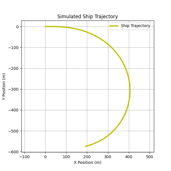
If you want, you can download the full code for this post here and play around with it.

---

Literature

Abkowitz, Martin A. Lectures on ship hydrodynamics—Steering and manoeuvrability. No. HY-5. 1964.

Fossen, Thor I. Handbook of marine craft hydrodynamics and motion control. John wiley & sons, 2011.

Yang, Youjun, Guillermo Chillcce, and Ould El Moctar. “Mathematical modeling of shallow water effects on ship maneuvering.” Applied Ocean Research 136 (2023): 103573.

Yang, Youjun, and Ould el Moctar. “A mathematical model for ships maneuvering in deep and shallow waters.” Ocean Engineering 295 (2024): 116927.