Rendering Fractals with WebGPU

What brought me here

I was always intrigued by fractals and their beautiful, intricate patterns that emerge just from simple mathematical rules. To explore them better and more interactively, I decided to build a fractal renderer, where you could zoom and move around the fractal in real-time. Since I am home to Python, my first try was, of course, write up a simple script using matplotlib to render the Mandelbrot set. This being arkwardly slow and non-interactive send me on a journey to explore WebGPU and how it can be used to render fractals blazingly fast in the browser.

In this post, I want to share this journey with you, and show how I implemented a simple fractal renderer using WebGPU. We will go through the basics of WebGPU, how to set up a rendering pipeline, and how to implement the Mandelbrot set rendering on the GPU. This is what we will be building:

But before we dive into the rendering part, let’s briefly talk about what fractals are and why they are so fascinating. We start with the Mandelbrot set.

The Mandelbrot Set

The Mandelbrot set is goverened by this simple quadratic map in the complex plane:

With the initial condition $z_0 = 0$, we can iterate this function to generate a sequence of complex numbers:

Mathematically, the Mandelbrot set is defined as the set of complex numbers $c$ for which the sequence does not diverge to infinity. More formally, a complex number $c$ is in the Mandelbrot set if there exists a constant $M$ such that for all $n$, $|z_n| \leq M$. In practice, we often use a threshold (commonly 2) to determine if the sequence diverges.

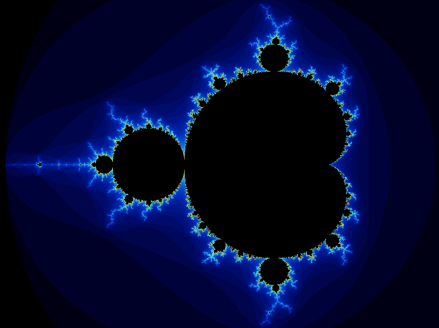
If we now were to perform this calculation for a grid of complex numbers in the complex plane, we can determine which points belong to the Mandelbrot set and which do not. By coloring the points based on how quickly they diverge, we can create a visual representation of the Mandelbrot set, revealing its intricate and beautiful structure:

The Julia Set

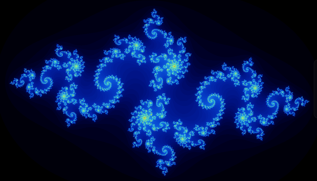
The Julia set is closely related to the Mandelbrot set and is defined by the same quadratic map, but with a fixed value of $c$ and varying initial conditions $z_0$. The Julia set for a given $c$ consists of all points in the complex plane that do not diverge when iterated through the function $f(z) = z^2 + c$. The shape of the Julia set can vary dramatically based on the value of $c$, and it can be connected or disconnected:

Other fractals

You can get all kinds of different fractals by changing the function we iterate. For example, the Burning Ship fractal is defined by the function:

But let’s not get ahead of ourselves. We focus on the Mandelbrot set for now, and will claim the Julia set basically for free since it’s the same code with a different parameter.

A naive rendering approach

Since JavaScript really isn’t my home turf, I will be using Python for the naive implementation, although we are tackling a web problem here.

Let us start simple. The easiest way to get a rendering of the Mandelbrot set is to just loop over a grid of complex numbers, perform the iteration for each point, and determine if it belongs to the set or not. This can be easily implemented in vanilla Python:

def mandelbrot_naive(c: complex, max_iter: int) -> int:    
    z = complex(0, 0)
    for i in range(max_iter):
        z = z * z + c
        if abs(z) > 2:
            return i
    return max_iter

if __name__ == "__main__":
    from time import perf_counter
    # Define the region of the complex plane to visualize
    x_min, x_max = -2.0, 1.0
    y_min, y_max = -1.5, 1.5
    width, height = 1920, 1080
    max_iter = 100

    # Create a grid of complex numbers
    x = [x_min + (x_max - x_min) * i / width for i in range(width)]
    y = [y_min + (y_max - y_min) * j / height for j in range(height)]
    
    # Compute the Mandelbrot set
    start_time = perf_counter()
    mandelbrot_set = [
        [mandelbrot_naive(complex(xi, yi), max_iter) 
            for xi in x] for yi in y]
    end_time = perf_counter()
    
    print(f"Time taken: {end_time - start_time:.2f} seconds")

Without any plotting, this code takes around 5 seconds to run on my Ryzen 7 3700X to produce a single frame. Given that we are perfoming around 2 million iterations (1920 $\times$ 1080), this is not too bad, but certainly isn’t anywhere near real-time. If we want to make this interactive, we need to speed it up drastically.

import numpy as np
import multiprocessing as mp

def apply_mandelbrot_map(c: complex, max_iterations: int) -> int:
    z = 0
    for i in range(max_iterations):
        z = z**2 + c
        if abs(z) > 2:
            return i
    return 0

def compute_row(args):
    row_index, re_values, im_values, max_iterations = args

    row_data = np.zeros(len(im_values), dtype=np.float32)
    real = re_values[row_index]

    for j, imag in enumerate(im_values):
        c = complex(real, imag)
        row_data[j] = apply_mandelbrot_map(c, max_iterations)

    return (row_index, row_data)

if __name__ == "__main__":
    from time import perf_counter
    res = (1920, 1080)

    # Prepare an empty image array.
    # Note: image[y, x] is typically the convention, so image has shape (height, width).
    image = np.zeros(res, dtype=np.float32)
    
    # Coordinate ranges (feel free to adjust).
    re = np.linspace(-2, 0.5, res[0])    # width direction
    im = np.linspace(-1.25, 1.25, res[1])  # height direction

    max_iter = 100

    # We’ll parallelize over the "rows"
    tasks = [(i, re, im, max_iter) for i in range(len(re))]

    with mp.Pool() as pool:
        start = perf_counter()
        results = pool.map(compute_row, tasks)
    for i, row_data in results:
        image[i,:] = row_data
    end = perf_counter()
    print(f"Time taken: {end - start:.2f} seconds")

We can, thus, conclude that we need something more powerful than just the CPU (with or without multiprocessing) to get real-time performance. You guessed it already: the GPU!

GPU rendering

Maybe we should start by a simple question: Why is the GPU so much faster than the CPU for certain tasks?

You can imagine the CPU as a highly versatile worker that can handle a wide variety of tasks, but it can only do a few things at the same time (limited number of cores). The GPU, on the other hand, is like a specialized assembly line designed to perform the same operation on many pieces of data simultaneously (thousands of cores). This makes the GPU particularly well-suited for tasks that can be parallelized, such as rendering graphics or performing large matrix operations. It achieves this speed because all of its cores work autonomously and in parallel, and do not depend on the results of each other. In contrast, the CPU often has to wait for one operation to finish before starting the next, which can create bottlenecks.

With this new knowledge aquired, we think of our problem of rendering the Mandelbrot set again. We have lots of points in the complex plane that we want to evaluate, and none of them depend on each other. Also, for every point, we are performing the same operation (iterating the function and checking for divergence). Sounds like a perfect candidate for GPU rendering!

Let’s see how we can leverage the GPU.

WebGPU

I started this project with absolute zero experience in graphics rendering or GPU programming, so I did a little google search find out how I could render graphics on the GPU and display them in the browser (so that I can share them with you). My little search left me with two options: WebGL and WebGPU. After some further research I stumbled upon an article from the developers of three.js (a popular JavaScript library for 3D graphics) that said WebGL get more and more outdated, and that WebGPU is the future of web graphics. So, based on this single article’s advice, I decided to go with WebGPU.

In the Figure below, you can see the basic interface of WebGPU:

We can see that WebGPU acts as a centralized communication layer between our application and the GPU. It abstracts away the complexities of different hardware and provides a unified API for developers to interact with the GPU. This means that we can write code that is portable across different platforms and devices, without needing to worry about the specifics of each GPU architecture.

Great, now to get going we will closely follow the first tutorial on webgpufundamentals.org, which covers basically everything we need for our task here.

We do this as soon as I find the time to write it up. The showcase is already up and running, I just need to write up the blog post.

Literature

WebGL - Official documentation for WebGL.

WebGPU - Official documentation for WebGPU.

Webgpufundamentals - A great resource to learn about WebGPU and how to use it for rendering graphics in the browser.

shader-tutorial.dev - A fantastic tutorial series that covers the basics of shader programming (although in GLSL).